R - Beginners Workshop: All in One View

Last updated on 2025-06-24 | Edit this page

Overview

Questions

What is this all about?

Objectives

Explain the general structure of this introductory course
Explain how to submit “homework” assignments

Introduction

This is the accompanying website to the Empra Differentielle Psychologie of Heidelberg University. It is authored and used by Sven Lesche. This course aims to cover:

Some R basics and how to structure code
Getting a first glimpse of data
Cleaning data
Running some analysis

Lesson Structure

The entire course is organized in short “Episodes” intended to take around 10-15mins to read and around 5-10mins to complete the challenges below. You will complete approximately one episode per week. At the end of each episode, you will upload a script containing the solutions to the challenges. The file format should be: lessonnumber_solutions_name_surname.R. Upload the script containing your solutions to a HeiBox folder and share that folder with me.

A word about Chat-GPT

Chat-GPT is an amazing tool that makes it much easier to just try something out. Importantly, it can take a lot of work off your hands, especially early on in your learning process. Most of the challenges here can just be solved by plugging them into a LLM like Chat-GPT. I encourage you to first try to find a solution yourself. You will learn a lot more by failing yourself first and continuing to try.

Nonetheless, sometimes it may be necessary to ask Chat-GPT or google a solution. In real data analysis, this is done a lot! Nobody knows anything. However, the most important thing for now is that you understand the code you write. Thus, if you use Chat-GPT, make it explain to you why this code works and what it is doing or ask it for hints instead of the solution.

Accompanying Material

This course relies heavily on R for Data Science (2e), which can be treated as an accompanying textbook.

Questions & Support

This is the first version of the new course material. If you have any questions or notice any inconsistencies / opportunities for improvement, feel free to reach out to to me via mail or Slack. If you feel comfortable using GitHub, also feel free to submit an issue.

Some opportunities for improvement are:

Is the material sufficiently explained? Can you follow?
Are the exercises too difficult / not enough to practice material learned in an episode?
Are you missing any information to complete following episodes?
Is there information missing or information that you do not require?
Are there any typos / wrong examples?
Whatever else comes to mind.

Feel free to reach out to me via any of the channels with your feedback. I will try to implement it as soon as possible. Thank you for your help in making this course better for coming students!

Key Points

Follow the structured outline to learn R basics and data analysis
Submit weekly scripts following the specified format
Contact me via mail or Slack for any queries

Content from R Setup

Last updated on 2025-06-24 | Edit this page

Overview

Questions

What is R, what is R Studio?
How to work with the R console and R scripts?
What is an R package?

Objectives

To gain familiarity with the various panes in the RStudio IDE
To gain familiarity with the buttons, short cuts and options in the RStudio IDE
To understand variables and how to assign to them
To be able to manage your workspace in an interactive R session
To be able to use mathematical and comparison operations
To be able to call functions
Introduction to package management

Introduction to RStudio

Welcome to the R portion of the Empra. This first lesson is adapted from resbaz’s introction to R workshop.

Throughout this lesson, you’re going to learn some of the fundamentals of the R language as well as some best practices for organizing code for scientific projects that will make your life easier.

We’ll be using RStudio: a free, open source R integrated development environment. It provides a built in editor, works on all platforms (including on servers) and provides many advantages such as integration with version control and project management.

Basic layout

When you first open RStudio, you will be greeted by three panels:

The interactive R console (entire left)
Environment/History (tabbed in upper right)
Files/Plots/Packages/Help/Viewer (tabbed in lower right)

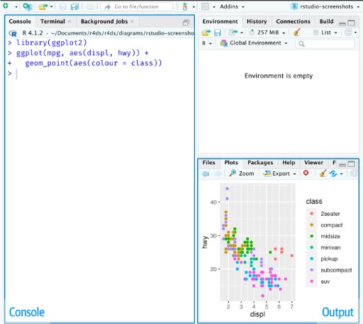
Once you open files, such as R scripts, an editor panel will also open in the top left.

Work flow within RStudio

There are two main ways one can work within RStudio.

Test and play within the interactive R console then copy code into a .R file to run later.
- This works well when doing small tests and initially starting off.
- It quickly becomes laborious
Start writing in an .R file - called a script - and use RStudio’s command / short cut to push current line, selected lines or modified lines to the interactive R console.
- This is a great way to start; all your code is saved for later
- You will be able to run the file you create from within RStudio or using R’s source() function.

For now, let’s stick with the console. We will learn more about how to use R scripts later. Feel free to run all code examples provided here in your own RStudio console and figure out what they do.

Introduction to the R console

Much of your time in R will be spent in the R interactive console. This is where you will run all of your code, and can be a useful environment to try out ideas before adding them to an R script file.

The first thing you will see in the R interactive session is a bunch of information, followed by a “>” and a blinking cursor. R operates on the idea of a “Read, evaluate, print loop”: you type in commands, R tries to execute them, and then returns a result.

Using R as a calculator

The simplest thing you could do with R is do arithmetic:

R

1 + 100

OUTPUT

[1] 101

And R will print out the answer, with a preceding “[1]”. Don’t worry about this for now, we’ll explain that later. For now think of it as indicating output.

If you type in an incomplete command, R will wait for you to complete it:

R

1 +

OUTPUT

Any time you hit return and the R session shows a “+” instead of a “>”, it means it’s waiting for you to complete the command. If you want to cancel a command you can simply hit “Esc” and RStudio will give you back the “>” prompt.

Tip: Cancelling commands

If you’re using R from the commandline instead of from within RStudio, you need to use Ctrl+C instead of Esc to cancel the command. This applies to Mac users as well!

Cancelling a command isn’t just useful for killing incomplete commands: you can also use it to tell R to stop running code (for example if its taking much longer than you expect), or to get rid of the code you’re currently writing.

When using R as a calculator, the order of operations is the same as you would have learnt back in school.

From highest to lowest precedence:

Parentheses: (, )
Exponents: ^ or **
Divide: /
Multiply: *
Add: +
Subtract: -

R

3 + 5 * 2

OUTPUT

[1] 13

Use parentheses to group operations in order to force the order of evaluation if it differs from the default, or to make clear what you intend.

R

(3 + 5) * 2

OUTPUT

[1] 16

This can get unwieldy when not needed, but clarifies your intentions. Remember that others may later read your code.

R

(3 + (5 * (2 ^ 2))) # hard to read
3 + 5 * 2 ^ 2       # clear, if you remember the rules
3 + 5 * (2 ^ 2)     # if you forget some rules, this might help

The text after each line of code is called a “comment”. Anything that follows after the hash (or octothorpe) symbol # is ignored by R when it executes code.

Really small or large numbers get a scientific notation:

R

2/10000

OUTPUT

[1] 2e-04

Which is shorthand for “multiplied by 10^XX”. So 2e-4 is shorthand for 2 * 10^(-4).

You can write numbers in scientific notation too:

R

5e3  # Note the lack of minus here

OUTPUT

[1] 5000

Mathematical functions

R has many built in mathematical functions. To call a function, we simply type its name, followed by open and closing parentheses. Anything we type inside the parentheses is called the function’s arguments:

R

sin(1)  # trigonometry functions

OUTPUT

[1] 0.841471

R

log(1)  # natural logarithm

OUTPUT

[1] 0

R

log10(10) # base-10 logarithm

OUTPUT

[1] 1

R

exp(0.5) # e^(1/2)

OUTPUT

[1] 1.648721

Don’t worry about trying to remember every function in R. You can simply look them up on Google, or if you can remember the start of the function’s name, use the tab completion in RStudio.

This is one advantage that RStudio has over R on its own, it has autocompletion abilities that allow you to more easily look up functions, their arguments, and the values that they take.

Typing a ? before the name of a command will open the help page for that command. As well as providing a detailed description of the command and how it works, scrolling to the bottom of the help page will usually show a collection of code examples which illustrate command usage. Try reading the description to the log() function by typing ?log() (or just ?log) in the console.

Comparing things

Another useful feature of R next to functions are comparisons. Quite often, we want to see if one value is bigger than another or only use data with some particular value.

We can check if two values are equal by using the equality operator ==.

R

1 == 1  # equality (note two equals signs, read as "is equal to")

OUTPUT

[1] TRUE

R

1 != 2  # inequality (read as "is not equal to")

OUTPUT

[1] TRUE

R

1 <  0  # less than

OUTPUT

[1] FALSE

R

1 <= 1  # less than or equal to

OUTPUT

[1] TRUE

R

1 > 1  # greater than

OUTPUT

[1] FALSE

R

1 >= 1 # greater than or equal to

OUTPUT

[1] TRUE

Variables and assignment

In the previous example, we simply used numbers to do comparisons. However, most work in R will be done using variables. A variable can be any quality, quantity or property we might be interested in, like a response time, a score on a personality test or a diagnosis. We can store values in variables using the assignment operator <-, like this:

R

x <- 1/40

Notice that assignment does not print a value. Instead, we stored it for later in something called a variable. x now contains the value 0.025:

R

OUTPUT

[1] 0.025

Look for the Environment tab in one of the panes of RStudio, and you will see that x and its value have appeared. Our variable x can be used in place of a number in any calculation that expects a number:

R

log(x)

OUTPUT

[1] -3.688879

Notice also that variables can be reassigned:

R

x <- 100

x used to contain the value 0.025 and and now it has the value 100.

We can also update the value of a variable and store it with the same name again.

R

x <- x + 1 #notice how RStudio updates its description of x on the top right tab

The right hand side of the assignment can be any valid R expression. The right hand side is fully evaluated before the assignment occurs. This means that in the above example, x + 1 is evaluated first and the result is only then assigned to the new x.

Variable names can contain letters, numbers, underscores and periods. They cannot start with a number nor contain spaces at all. Different people use different conventions for long variable names, these include

periods.between.words
underscores_between_words
camelCaseToSeparateWords

What you use is up to you, but be consistent.

R

this_is_okay

this.is.also.okay

someUseCamelCase

dont_be.aMenace_toSociety

I always use snake_case for variable names in R. camelCase is often used in other programming languages such as MATLAB or JavaScript.

Using = for assignment

It is also possible to use the = operator for assignment:

R

x = 1/40

But this is much less common among R users. The most important thing is to be consistent with the operator you use. There are occasionally places where it is less confusing to use <- than =, and it is the most common symbol used in the community. So the recommendation is to use <-.

If we try to give a variable an invalid name, R will throw an error.

R

2_times_x = 2*x

ERROR

Error in parse(text = input): <text>:1:2: unexpected input
1: 2_
     ^

Tip: Warnings vs. Errors

Pay attention when R does something unexpected! Errors, like above, are thrown when R cannot proceed with a calculation. Warnings on the other hand usually mean that the function has run, but it probably hasn’t worked as expected.

In both cases, the message that R prints out usually give you clues how to fix a problem.

Errors can be frustrating, but they are your friend! They tell you that something went wrong and usually give you an informative message as to what went wrong. If you cannot make something of the error message, try pasting it into Google or Chat-GPT, this will often help.

Challenges

Challenge 1

Which of the following are valid R variable names? Feel free to try them all out in R and figure out which produce errors and why.

R

min_height
max.height
_age
.mass
MaxLength
min-length
2widths
celsius2kelvin

Challenge 2

What will be the value of each variable after each statement in the following program? You are encouraged to run these commands in R.

R

mass <- 47.5
age <- 122
mass <- mass * 2.3
age <- age - 20

Challenge 3

Run the code from the previous challenge, and write a command to compare mass to age. Is mass larger than age?

Key Points

R Studio is a shiny environment that helps you write R code
You can either write code directly in the console, or use script to organize and save your code
You can assign variables using <-
Be consistent in naming variables, other people should be able to read and understand your code

Content from Packages in R

Last updated on 2025-06-24 | Edit this page

Overview

Questions

What is an R package?
How can we use R packages

Objectives

Explain how to use R packages
Explain how to install R packages
Understand the difference between installing and loading an R package

R Packages

Per default, R provides you with some basic functions like sum(), mean() or t.test(). These functions can already accomplish a lot, but for more specialized analyses or more user-friendly functions, you might want to use additional functions.

If you are in need of a specific function to achieve your goal, you can either write it yourself (more on this later) or use functions written by other users. These functions are often collected in so-called “packages”. The official source for these packages on R is CRAN (the comprehensive R archive network).

Packages you may encounter

Packages make R really powerful. For 95% of your analysis-needs, there probably exists a package designed specifically to hand this. For example, some packages you might use often are tidyverse for data cleaning, psych for some psychology specific functions, afex for ANOVAs or lme4 for multi-level models. You can even use R packages for more complicated analyses like structural equation models (lavaan) or bayesian modeling (brms). You can even write papers using R using papaya. Even this website was written using the R-packages rmarkdown and sandpaper.

CRAN makes it really easy to use the over 7000 R packages other users provide. You can install them using install.packages("packagename") with the name of the package in quotation marks. This installs all functionalities of this packages on your machine. However, this package is not automatically available to you. Before using it in a script (or the console) you need to tell R to “activate” this package. You can do this using library(packagename). This avoids loading all installed packages every time R is starting (which would take a while).

Using functions without loading a package

If you are only using a few functions from a certain package (maybe even only once), you can avoid loading the entire package and only specifically access that function using the :: operator. You can do this by typing packagename::function(). If the package is installed, it will allow you to use that function without calling library(packagename) first. This may also be useful in cases where you want to allow the reader of your code to easily understand what package you used for a certain function.

Demonstration

First, we need to install a package. This will often generate a lot of text in your console. This is nothing to worry about. In most cases, it is enough to look at the last few messages, they will tell you what went wrong or whether everything went right.

R

install.packages("dplyr")

OUTPUT

The following package(s) will be installed:
- dplyr [1.1.4]
These packages will be installed into "~/work/r-for-empra/r-for-empra/renv/profiles/lesson-requirements/renv/library/linux-ubuntu-jammy/R-4.5/x86_64-pc-linux-gnu".

# Installing packages --------------------------------------------------------
- Installing dplyr ...                          OK [linked from cache]
Successfully installed 1 package in 4.9 milliseconds.

Then, we will need to load the package to make its functions available for use. For most packages, this will also print a lot of messages in the console in the bottom left. Again, this is usually harmless. If something does go wrong, you will see the word Error: along with a message somewhere. Warnings: can often be ignored in package installation.

R

# Loading the package dplyr
library(dplyr)

OUTPUT


Attaching package: 'dplyr'

OUTPUT

The following objects are masked from 'package:stats':

    filter, lag

OUTPUT

The following objects are masked from 'package:base':

    intersect, setdiff, setequal, union

Now we can use all the functions that dplyr provides. Let’s start by using glimpse() to get a quick glance at some data. For this case, we are using the iris data, that comes with your default R installation.

R

# iris is a dataset provided as default in R
glimpse(iris)

OUTPUT

Rows: 150
Columns: 5
$ Sepal.Length <dbl> 5.1, 4.9, 4.7, 4.6, 5.0, 5.4, 4.6, 5.0, 4.4, 4.9, 5.4, 4.…
$ Sepal.Width  <dbl> 3.5, 3.0, 3.2, 3.1, 3.6, 3.9, 3.4, 3.4, 2.9, 3.1, 3.7, 3.…
$ Petal.Length <dbl> 1.4, 1.4, 1.3, 1.5, 1.4, 1.7, 1.4, 1.5, 1.4, 1.5, 1.5, 1.…
$ Petal.Width  <dbl> 0.2, 0.2, 0.2, 0.2, 0.2, 0.4, 0.3, 0.2, 0.2, 0.1, 0.2, 0.…
$ Species      <fct> setosa, setosa, setosa, setosa, setosa, setosa, setosa, s…

R

# Using a function without loading the entire package
# dplyr::glimpse(iris)

Here, we can see that iris has 150 rows (or observations) and 5 columns (or variables). The first four variables are size measurements regarding length and width of sepal and petal and the fifth variable is a variable containing the species of flower.

Challenges

Challenge 1:

Install the following packages: dplyr, ggplot2, and psych.

Challenge 2:

Load the package dplyr and get an overview of the data mtcars using glimpse().

Challenge 3:

Figure out what kind of data mtcars contains. Make a list of the columns in the dataset and what they might mean.

Hint

You are allowed to use Google (or other sources) for this. It is common practice to google information you don’t know or look online for code that might help.

Challenge 4:

Use the function describe() from the package psych without loading it first.

What differences do you notice between glimpse() and describe()?

Key Points

R packages are “add-ons” to R, they provide useful new tools.
Install a package using install.packages("packagename").
Use a package using library(packagename) at the beginning of your script.
Use :: to access specific functions from a package without loading it entirely.

Content from Vectors and variable types

Last updated on 2025-06-24 | Edit this page

Overview

Questions

How do you use scripts in R to document your work?
How can you organize scripts effectively?
What is a vector?

Objectives

Show how to use scripts to generate reproducible analyses
Explain what a vector is
Explain variable types
Show examples of sum() and mean()

Scripts in R

For now, we have been only using the R console to execute commands. This works great if there are some quick calculations you have to run, but is unsuited for more complex analyses. If you want to reproduce the exact steps you took in data cleaning and analyses, you need to write them down - like a recipe.

This is where R scripts come in. They are basically like a text file (similar to Word) where you can write down all the steps you took. This makes it possible to retrace them and produce the exact same result over and over again.

In order to use R scripts effectively, you need to do two things. Firstly, you need to write them in a way that is understandable in the future. We will learn more about how to write clean code in future lessons. Secondly (and maybe more importantly) you need to actually save these scripts on your computer, and ideally save them in a place where you can find them again. The place where you save your script and especially the place you save your data should ideally be a folder in a sensible place. For example, this script is saved in a sub-folder episodes/ of the workshop folder r_for_empra/. This makes it easy for humans to find the script. Aim for similar clarity in your folder structure!

For this lesson, create a folder called r_for_empra somewhere on your computer where it makes sense for you. Then, create a new R script by clicking File > New File > R Script or hitting Ctrl + Shift + N. Save this script as episode_scripts_and_vectors.R in the folder r_for_empra created above. Follow along with the episode and note down the commands in your script.

Using a script

Let’s start learning about some basic elements of R programming. We have already tried assigning values to variables using the <- operator. For example, we might assign the constant km_to_m the value 1000.

R

km_to_m <- 1000

Now, if we had data on distances in km, we could also use this value to compute the distance in meters.

R

distance_a_to_b_km <- 7.56

distance_a_to_b_m <- distance_a_to_b_km * km_to_m

If we have multiple distances and want to transform them from km to m at the same time, we can make use of a vector. A vector is just a collection of elements. We can create a vector using the function c() (for combine).

Tip: Running segments of your code

RStudio offers you great flexibility in running code from within the editor window. There are buttons, menu choices, and keyboard shortcuts. To run the current line, you can 1. click on the Run button just above the editor panel, or 2. select “Run Lines” from the “Code” menu, or 3. hit Ctrl + Enter in Windows or Linux or Command-Enter on OS X. (This shortcut can also be seen by hovering the mouse over the button). To run a block of code, select it and then Run via the button or the keyboard-shortcut Ctrl + Enter.

Variable Types

Vectors can only contain values of the same type. There are two basic types of variables that you will have to interact with - numeric and character variables. Numeric variables are any numbers, character variables are bits of text.

R

# These are numeric variables:
vector_of_numeric_variables <- c(4, 7.642, 9e5, 1/97) # recall, 9e5 = 9*10^5

# Show the output
vector_of_numeric_variables

OUTPUT

[1] 4.000000e+00 7.642000e+00 9.000000e+05 1.030928e-02

R

# These are character variables:
vector_of_character_variables <- c("This is a character variable", "A second variable", "And another one")

# Show the output
vector_of_character_variables

OUTPUT

[1] "This is a character variable" "A second variable"
[3] "And another one"

We can not only combine single elements into a vector, but also combine multiple vectors into one long vector.

R

numeric_vector_1 <- c(1, 2, 3, 4, 5)
numeric_vector_2 <- c(6:10) # 6:10 generates the values 6, 7, 8, 9, 10

combined_vector <- c(numeric_vector_1, numeric_vector_2)
combined_vector

OUTPUT

 [1]  1  2  3  4  5  6  7  8  9 10

Recall that all elements have to be of the same type. If you try to combine numeric vectors with character vectors, R will automatically convert everything to a character vector (as this has less restrictions, anything can be a character).

R

character_vector_1 <- c("6", "7", "8")
# Note that the numbers are now in quotation marks!
# They will be treated as characters, not numerics!

combining_numeric_and_character <- c(numeric_vector_1, character_vector_1)
combining_numeric_and_character

OUTPUT

[1] "1" "2" "3" "4" "5" "6" "7" "8"

We can fix this issue by converting the vectors to the same type. Note how the characters are also just numbers, but in quotation marks. Sometimes, this happens in real data, too. Some programs store every variable as a character (sometimes also called string). We then have to convert the numbers back to the number format:

R

converted_character_vector_1 <- as.numeric(character_vector_1)

combining_numeric_and_converted_character <- c(numeric_vector_1, converted_character_vector_1)

combining_numeric_and_converted_character

OUTPUT

[1] 1 2 3 4 5 6 7 8

But be careful, this conversion does not always work! If R does not know how to convert a specific character to a number, it will simply replace this with NA.

R

character_vector_2 <- c("10", "11", "text")
# The value "text", can not be interpreted as a number

as.numeric(character_vector_2)

WARNING

Warning: NAs introduced by coercion

OUTPUT

[1] 10 11 NA

Inspecting the type of a variable

You can use the function str() to learn about the structure of a variable. The first entry of the output tells us about the type of the variable.

R

str(vector_of_numeric_variables)

OUTPUT

 num [1:4] 4.00 7.64 9.00e+05 1.03e-02

This tells us that there is a numeric vector, hence num, with 4 elements.

R

str(vector_of_character_variables)

OUTPUT

 chr [1:3] "This is a character variable" "A second variable" ...

This tells us that there is a character vector, hence chr, with 3 elements.

R

str(1:5)

OUTPUT

 int [1:5] 1 2 3 4 5

Note that this prints int and not the usual num. This is because the vector only contains integers, so whole numbers. These are stored in a special type that takes up less memory, because the numbers need to be stored with less precision. You can treat it as very similar to a numeric vector, and do all the same wonderful things with it!

Simple functions for vectors

Let’s use something more exciting than a sequence from 1 to 10 as an example vector. Here, we use the mtcars data that you already got to know in an earlier lesson. mtcars carries information about cars, like their name, fuel usage, weight, etc. This information is stored in a data frame. A data frame is a rectangular collection of variables (in the columns) and observations (in the rows). In order to extract vectors from a data frame we can use the $ operator. data$column extracts a vector.

R

mtcars_weight_tons <- mtcars$wt 

# note that it is a good idea to include the unit in the variable name
mtcars_weight_tons

OUTPUT

 [1] 2.620 2.875 2.320 3.215 3.440 3.460 3.570 3.190 3.150 3.440 3.440 4.070
[13] 3.730 3.780 5.250 5.424 5.345 2.200 1.615 1.835 2.465 3.520 3.435 3.840
[25] 3.845 1.935 2.140 1.513 3.170 2.770 3.570 2.780

Let’s start learning some basic information about this vector:

R

str(mtcars_weight_tons)

OUTPUT

 num [1:32] 2.62 2.88 2.32 3.21 3.44 ...

The vector is of type numeric and contains 32 entries. We can double check this by looking into our environment tab, where num [1:32] indicates just that. Similarly, we can get the length of a vector by using length()

R

length(mtcars_weight_tons)

OUTPUT

[1] 32

We can compute some basic descriptive information of the weight of cars in the mtcars data using base-R functions:

R

# Mean weight:
mean(mtcars_weight_tons)

OUTPUT

[1] 3.21725

R

# Median weight:
median(mtcars_weight_tons)

OUTPUT

[1] 3.325

R

# Standard deviation:
sd(mtcars_weight_tons)

OUTPUT

[1] 0.9784574

To get the minimum and maximum value, we can use min() and max().

We can also get a quick overview of the weight distribution using hist(), which generates a simple histogram.

R

hist(mtcars_weight_tons)

Histograms

Histograms are more powerful tools than it seems on first glance. They allow you to simply gather knowledge about the distribution of your data. This is especially important for us psychologists. Do we have ceiling effects in the task? Were some response options even used? How is response time distributed?

If your histogram is not detailed enough, try adjusting the breaks parameter. This tells hist() how many bars to print in the plot.

R

hist(mtcars_weight_tons, breaks = 30)

The golden rule for the number of breaks is simple: try it until it looks good! You are free to explore here.

Another useful function is unique(). This function removes duplicates and only returns unique values. I use it a lot in experimental data. Since every participant contributes multiple trials, but I am sometimes interested in values a participant only contributes once, I can use unique() to only retain each value once.

In mtcars data, we might want to see how many cylinders are possible in the data. unique(mtcars$cyl) is much easier to read at a glance.

R

mtcars$cyl

OUTPUT

 [1] 6 6 4 6 8 6 8 4 4 6 6 8 8 8 8 8 8 4 4 4 4 8 8 8 8 4 4 4 8 6 8 4

R

unique(mtcars$cyl)

OUTPUT

[1] 6 4 8

Tip: Unique + Length = Quick Count

Combining unique() and length() leads to a really useful property. This returns the number of unique entries in a vector. I use it almost daily! For example to figure out how many participants are in a given data frame. unique(data$participant_id) returns all the different participant ids and length(unique(data$participant_id)) then gives me the number of different ids, so the number of participants in my data.

Indexing and slicing vectors

There is one more important thing to learn about vectors before we move on to more complicated data structures. Most often, you are going to use the whole vector for computation. But sometimes you may only want the first 150 entries, or only entries belonging to a certain group. Here, you must be able to access specific elements of the vector.

In the simplest case, you can access the $n$th element in a vector by using vector[n]. To access the first entry, use vector[1], and so on.

R

test_indexing_vector <- seq(1, 32, 1) 
# Seq generates a sequence from the first argument (1) to the second argument (32) 
# The size of the steps is given by the third argument

test_indexing_vector

OUTPUT

 [1]  1  2  3  4  5  6  7  8  9 10 11 12 13 14 15 16 17 18 19 20 21 22 23 24 25
[26] 26 27 28 29 30 31 32

R

test_indexing_vector[1]

OUTPUT

[1] 1

R

test_indexing_vector[c(1, 2)]

OUTPUT

[1] 1 2

You can also remove an element (or multiple) from a vector by using a negative sign -.

R

test_indexing_vector[-c(11:32)] # this removes all indexes from 11 to 32

OUTPUT

 [1]  1  2  3  4  5  6  7  8  9 10

The same rules apply for all types of vectors (numeric and character).

Tip: Think about the future

Excluding by index is a simple way to clean vectors. However, think about what happens if you accidentally run the command vector <- vector[-1] twice, instead of once?

Show me the solution

The first element is going to be excluded twice. This means that the vector will lose two elements. In principle, it is a good idea to write code that you can run multiple times without causing unwanted issues. To achieve this, either use a different way to exclude the first element that we will talk about later, or simply assign the cleaned vector a new name:

R

cleaned_vector <- vector[-1]

Now, no matter how often you run this piece of code, cleaned_vector will always be vector without the first entry.

Filtering vectors

In most cases, you don’t know what the element of the vector is you want to exclude. You might know that some values are impossible or not of interest, but don’t know where they are. For example, the accuracy vector of a response time task might look like this:

R

accuracy_coded <- c(0, 1, 1, 1, 1, -2, 99, 1, 11, 0)
accuracy_coded

OUTPUT

 [1]  0  1  1  1  1 -2 99  1 11  0

-2 and 99 are often used to indicate invalid button-presses or missing responses. 11 in this case is a wrong entry that should be corrected to 1.

If we were to compute the average accuracy now using mean() we would receive a wrong response.

R

mean(accuracy_coded)

OUTPUT

[1] 11.3

Therefore, we need to exclude all invalid values before continuing our analysis. Before I show you how I would go about doing this, think about it yourself. You do not need to know the code, yet. Just think about some rules and steps that need to be taken to clean up the accuracy vector. What comparisons could you use?

Important: The silent ones are the worst

The above example illustrates something very important. R will not throw an error every time you do something that doesn’t make sense. You should be really careful of “silent” errors. The mean() function above works exactly as intended, but returns a completely nonsensical value. You should always conduct sanity checks. Can mean accuracy be higher than 1? How many entries am I expecting in my data?

Now, back to the solution to the wacky accuracy data. Note that R gives us the opportunity to do things in a million different ways. If you came up with something different from what was presented here, great! Make sure it works and if so, use it!

First, we need to recode the wrong entry. That 11 was supposed to be a 1, but someone entered the wrong data in the excel. To do this, we can find the index, or the element number, where accuracy is 11. Then, we can replace that entry with 1.

R

index_where_accuracy_11 <- which(accuracy_coded == 11)

accuracy_coded[index_where_accuracy_11] <- 1
# or in one line:
# accuracy_coded[which(accuracy_coded == 11)] <- 1

accuracy_coded

OUTPUT

 [1]  0  1  1  1  1 -2 99  1  1  0

Now, we can simply exclude all values that are not equal to 1 or 0. We do this using the - operators:

R

accuracy_coded[-which(accuracy_coded != 0 & accuracy_coded != 1)]

OUTPUT

[1] 0 1 1 1 1 1 1 0

However, note that this reduces the number of entries we have in our vector. This may not always be advisable. Therefore, it is often better to replace invalid values with NA. The value NA (not available) indicates that something is not a number, but just missing.

R

# Note that now we are not using the - operator
# We want to replace values that are not 0 or 1
accuracy_coded[which(accuracy_coded != 0 & accuracy_coded != 1)] <- NA

Now, we can finally compute the average accuracy in our fictional experiment.

R

mean(accuracy_coded)

OUTPUT

[1] NA

Challenges

Challenge 1:

We did not get a number in the above code. Figure out why and how to fix this. You are encourage to seek help on the internet.

Challenge 2:

Below is a vector of response times. Compute the mean response time, the standard deviation, and get the number of entries in this vector.

R

response_times_ms <- c(
  230.7298, 620.6292, 188.8168, 926.2940, 887.4730,
  868.6299, 834.5548, 875.2154, 239.7057, 667.3095,
  -142.891, 10000, 876.9879
  )

Challenge 3:

There might be some wrong values in the response times vector from above. Use hist() to inspect the distribution of response times. Figure out which values are implausible and exclude them. Recompute the mean response time, standard deviation, and the number of entries.

Challenge 4:

Get the average weight (column wt) of cars in the mtcars data . Can you spot any outliers in the histogram?

Exclude the “outlier” and rerun the analyses.

Challenge 5:

Get the mean values of responses to this fictional questionnaire:

R

item_15_responses <- c("1", "3", "2", "1", "2", "none", "4", "1", "3", "2", "1", "1", "none")

Challenge 6 (difficult):

Compute the average of responses that are valid as indicated by the vector is_response_valid:

R

response_values <- c(91, 82, 69, 74, 62, 19, 84, 61, 92, 53)
is_response_valid <- c("yes", "yes", "yes", "yes", "yes",
                       "no", "yes", "yes", "yes", "no")

Show me the solution

R

valid_responses <- response_values[which(is_response_valid == "yes")]
mean(valid_responses)

OUTPUT

[1] 76.875

Key Points

Scripts facilitate reproducible research
create vectors using c()
Numeric variables are used for computations, character variables often contain additional information
You can index vectors by using vector[index] to return or exclude specific indices
Use which() to filter vectors based on specific conditions

Content from Projects

Last updated on 2025-06-24 | Edit this page

Overview

Questions

What is an R project?
How do projects help me organize my scripts.

Objectives

Explain how projects can provide structure
Explain what a “working directory” is and how to access files

Working Directory

Last week we worked with scripts and some basic computations using vectors. Most likely, you wrote down a lot of code and saved the script somewhere on your computer. Once you start working with multiple scripts and datasets, it becomes very important that you keep your files somewhat orderly.

This is important both for us humans to understand, but also for computers. Any time you need to access something outside your present R script, you will need to tell R where to find this. The data will be saved somewhere on the computer and needs to find its way into the R session.

Understanding where a file is saved on your computer is key to understanding how to tell R to read it into your current session. There are two main ways to tell R how to find a file: absolute paths and relative paths.

Absolute Paths

An absolute path is the full location of a file on your computer, starting from the root of your file system. It tells R exactly where to find the file, no matter where your R script is located. Think of it like an address in a town. 1404 Mansfield St, Chippewa Falls, WI 54729 tells you exactly where a house is located.

For example, the absolute path to a file stored in the Documents/ folder most likely looks something like this:

Windows: "C:/Users/YourName/Documents/my_data.csv"
Mac/Linux: "/Users/YourName/Documents/my_data.csv"

How to Find the Absolute Path of a File:

On Windows, open File Explorer, navigate to your file, right-click it, and select Properties. The full file path will be shown in the “Location” field.
On Mac, open Finder, right-click the file, select Get Info, and look at “Where.”

Relative Paths

A relative path specifies the location of a file in relation to the working directory of your R session. This is useful when working with projects that contain multiple files, as it keeps your code flexible and portable. Think of this like the direction, “just follow the road until the roundabout and then take the second exit”. If the starting point is well defined, this is enough information to find the target.

The working directory is the default folder on your computer where R looks for files and saves new ones. Think of it as R’s “home base”—if you ask R to read or save a file without giving a full path, it will assume you’re talking about this location.

You can check your current working directory by running:

R

getwd()  # This tells you where R is currently looking for files

OUTPUT

[1] "/home/runner/work/r-for-empra/r-for-empra/site/built"

In our case, this means if you try to read a file like this:

R

read.csv("data.csv")

R will look for data.csv inside /home/runner/work/r-for-empra/r-for-empra/site/built.

If your files are stored somewhere else, you can change the working directory using:

R

setwd("C:/Users/YourName/Desktop/MyNewFolder")  # Set a new working directory

Now, R will assume all file paths start from "C:/Users/YourName/Desktop/MyNewFolder".

There are two main ways to define the working directory that R will use. You can do this using setwd() and specify a particular directory you want to start from. Another way to accomplish this is through the use of R projects. These projects automatically set your working directory to the place that the project is located. More about projects in just a second.

If you prefer declaring your working directory using setwd(), you can place this bit of code setwd(dirname(rstudioapi::getActiveDocumentContext()$path)) at the beginning of your script. R will then set the working directory to the folder that the script you are working with is located in.

Why is the Working Directory Important?

It saves you from typing long file paths every time you load data.
It keeps projects organized by ensuring all files are in a central location.
It makes your code portable, so if you share your project, others won’t need to change file paths manually.

R Projects

I do not recommend using setwd(). Instead, I would suggest using R projects. When working in RStudio, using R Projects is one of the best ways to keep your work organized, portable, and efficient. An R Project is essentially a self-contained workspace that helps manage files, working directories, and settings automatically.

There are several reasons why I prefer R projects:

1️⃣ Automatic Working Directory Management

When you open an R Project, RStudio automatically sets the working directory to the project’s folder. This means you don’t have to use setwd() manually or worry about absolute file paths.

Example:
- If your project folder is C:/Users/YourName/Documents/MyProject, then any file in this folder can be accessed with a relative path:

R

read.csv("data/my_data.csv")  # No need for long paths!

2️⃣ Keeps Everything Organized

An R Project keeps all related files—scripts, datasets, plots, and outputs—in one place. This is especially useful when working on multiple projects, preventing files from getting mixed up.

A typical project folder might look like this:

MyProject/
│── data/         # Raw data files
│── scripts/      # R scripts
│── output/       # Processed results
│── MyProject.Rproj  # The project file

This structure helps keep your work clean and easy to navigate.

3️⃣ Easier Collaboration & Portability

If you share your project folder, others can open the .Rproj file in RStudio and immediately start working—no need to change file paths or set up the environment manually. This makes R Projects ideal for:
✅ Teamwork
✅ Sharing with collaborators
✅ Reproducible research

4️⃣ Integrated Version Control (Git)

If you use Git for version control, R Projects make it simple to track changes, commit updates, and collaborate through platforms like GitHub. You can set up a Git repository directly inside the project.

5️⃣ Easy Switching Between Projects

With R Projects, you can quickly switch between different tasks without affecting the working directory or opening and closing scripts. Each project remembers its settings, so you don’t have to reconfigure things every time.

How to Create an R Project

1️⃣ Open RStudio
2️⃣ Click File → New Project
3️⃣ Choose New Directory (or an existing folder)
4️⃣ Select New Project and give it a name
5️⃣ Click Create Project 🎉

Now, whenever you open the .Rproj file, RStudio will automatically set everything up for you!

You can open a project using File > Open Project in the top left of R Studio. You will then notice the projects name appearing in the top right. Furthermore, the Files view in the bottom right will automatically go to the destination of your selected project.

Creating an R project

Let’s go through the steps of setting up an R project together. First, decide if you want to use an existing folder or generate a brand new folder for your R project. I would suggest using a folder that is clean. For example, use the folder r_for_empra that you created a couple lessons earlier!

To create a project, follow the steps outlined above. Make sure the creation of your project was successful and you can see the name of your project in the top right corner. If you are creating the project in a new folder, you will have to give it a sensible name!

Challenges

Challenge 1:

Make sure you have the project created. In the folder that the project is created in, add the following sub-folders: data, processed_data and archive. You can do this either in the file explorer of your computer, or by using the bottom right window of RStudio.

data will house all the raw data files that we are working with in this tutorial. processed_data will be used to save data that we processed in some way and want to reuse later on. archive is a folder to store old scripts or data-sets that you will no longer use. You can also delete those files, but I often find it easier to just “shove them under the bed” so that I could still use them later on.

Get an overview of the folders in your project by running list.dirs(recursive = FALSE). This should return the folders you just created and a folder where R-project information is stored.

If you do not see the folders you just created, make sure you created and opened the project and that the folders are in the same space as your .Rproj project file.

Challenge 2:

Download the following data and place it in the data folder. Make sure to give it an appropriate name. The data contains information about the number of times the character Roy Kent used the f-word in the show Ted Lasso.

Challenge 3:

Test the data you just downloaded. Read it into R and give it an appropriate name.

Hint: You may need to research how to read .csv files into R first.

Show me the solution

R

roy_kent_data <- read.csv("data/roy_kent_f_count.csv")

Challenge 4:

Familiarize yourself with the data. What columns are there (use colnames(data)). Compute the average amount of times Roy Kent says “Fuck” in an episode. Compute the total amount of times he said it throughout the series.

Show me the solution

R

average_f_count <- mean(roy_kent_data$F_count_RK)
total_f_count <- sum(roy_kent_data$F_count_RK)

# Because, cum_rk_overall is a running (cumulative) total:
total_f_count <- max(roy_kent_data$cum_rk_overall)

Key Points

The working directory is where R looks for and saves files.
Absolute paths give full file locations; relative paths use the working directory.
R Projects manage the working directory automatically, keeping work organized.
Using R Projects makes code portable, reproducible, and easier to share.
A structured project with separate folders for data and scripts improves workflow.

Content from Data Visualization (1)

Last updated on 2025-06-24 | Edit this page

Overview

Questions

How can you get an overview of data?
How do you visualize distributions of data?

Objectives

Learn how to read in .csv files
Learn how to explore a dataset for the first time
Learn how to visualize key statistics of data

Reading in data

You already had to read in data in the last lesson. Data comes in many shapes and sizes. The format of data you had to read in the last session is called csv, for comma-separated values. This is one of the most common data formats. It gets its name because all values are separated from each other using a comma “,”. Here in Germany, csv files are sometimes separated by a semicolon “;” instead. This can be adjusted in R-code by using read.csv("path/to/file", sep = ";") and declaring the semicolon as the separating variable.

Reading data requires specific functions

There are several other common formats including .xlsx for excel files, .sav for SPSS files, .txt for simple text files and .rdata for a special R-specific data format. These files can not be read in by read.csv(), as this is only for .csv files. Instead, use specific functions for each format like readxl::read_excel(), or haven::read_sav().

Let’s again read in the data about Roy Kent’s potty-mouth.

R

roy_kent_data <- read.csv("data/roy_kent_f_count.csv")

Getting a glimpse of the data

When starting out with some data you received, it is important to familiarize yourself with the basics of this data first. What columns does it have, what information is contained in each row? What do the columns mean?

One option to get a quick overview of the data is… just looking at it! By clicking on the data in the Environment tab or typing View(roy_kent_data) in the console, you can inspect the data in R Studio. This will already show you how many observations (in this case rows) and variables (columns) the data has. We can also inspect the column names and see the first few entries. Look at the data, what might each column represent?

Now, let’s go back to using programming to inspect data. We already learned about the handy function glimpse(), for which we need the dplyr package.

R

library(dplyr)

glimpse(roy_kent_data)

OUTPUT

Rows: 34
Columns: 16
$ Character         <chr> "Roy Kent", "Roy Kent", "Roy Kent", "Roy Kent", "Roy…
$ Episode_order     <int> 1, 2, 3, 4, 5, 6, 7, 8, 9, 10, 11, 12, 13, 14, 15, 1…
$ Season            <int> 1, 1, 1, 1, 1, 1, 1, 1, 1, 1, 2, 2, 2, 2, 2, 2, 2, 2…
$ Episode           <int> 1, 2, 3, 4, 5, 6, 7, 8, 9, 10, 1, 2, 3, 4, 5, 6, 7, …
$ Season_Episode    <chr> "S1_e1", "S1_e2", "S1_e3", "S1_e4", "S1_e5", "S1_e6"…
$ F_count_RK        <int> 2, 2, 7, 8, 4, 2, 5, 7, 14, 5, 11, 10, 2, 2, 23, 12,…
$ F_count_total     <int> 13, 8, 13, 17, 13, 9, 15, 18, 22, 22, 16, 22, 8, 6, …
$ cum_rk_season     <int> 2, 4, 11, 19, 23, 25, 30, 37, 51, 56, 11, 21, 23, 25…
$ cum_total_season  <int> 13, 21, 34, 51, 64, 73, 88, 106, 128, 150, 16, 38, 4…
$ cum_rk_overall    <int> 2, 4, 11, 19, 23, 25, 30, 37, 51, 56, 67, 77, 79, 81…
$ cum_total_overall <int> 13, 21, 34, 51, 64, 73, 88, 106, 128, 150, 166, 188,…
$ F_score           <dbl> 0.1538462, 0.2500000, 0.5384615, 0.4705882, 0.307692…
$ F_perc            <dbl> 15.4, 25.0, 53.8, 47.1, 30.8, 22.2, 33.3, 38.9, 63.6…
$ Dating_flag       <chr> "No", "No", "No", "No", "No", "No", "No", "Yes", "Ye…
$ Coaching_flag     <chr> "No", "No", "No", "No", "No", "No", "No", "No", "No"…
$ Imdb_rating       <dbl> 7.8, 8.1, 8.5, 8.2, 8.9, 8.5, 9.0, 8.7, 8.6, 9.1, 7.…

This will tell us the variable type of each column, too. We can see that the first column is a character column which just contains the name of the hero of this data Roy Kent. The second column is an integer (so whole numbers) vector with information about the episode number.

Next, let’s try to figure out what each of the column names mean and what type of information is stored here. Some columns are self-explanatory like Season or Episode. Others might require a bit of background knowledge like Imdb_rating, which requires you to know about the film-rating platform “Imdb”.

Some columns are riddled with abbreviations that make their names easier to write, but harder to understand. F_count_RK is using RK as an abbreviation of Roy Kent and F as an abbreviation for… something else. cum_rk_overall is a cumulative (running) total of the number of times Roy used the F-word.

Yet other columns are really difficult to understand, because the implication is not 100% clear. What does F_count_total mean? The number of times “Fuck” was said in an episode? Seems like a reasonable guess, but in order to be sure, it’s best if we had some documentation of the data’s author’s intentions. This is often called a codebook, where the person compiling data writes down information about the meaning of column names, cleaning procedures and other oddities of the data. When sharing your own data online, this is essential in order to make your data useable for others.

There is no codebook included in this workshop, but you can find it online. The data is taken from an event called “Tidy-Tuesday”, a weekly event about cleaning and presenting interesting data using R. You can find information about the Roy Kent data here. Give it a read in order to make sure you know what all the columns are about.

Inspecting important values

Now that we understand the structure of the data and the names of the columns, we can start getting a look at the data itself. A good way to get an overview of data with loads of numeric variables is psych::describe(). This outputs you some basic descriptive statistics of the data.

R

psych::describe(roy_kent_data) # describe() function from psych package

OUTPUT

                  vars  n   mean     sd median trimmed    mad   min    max
Character*           1 34   1.00   0.00   1.00    1.00   0.00  1.00   1.00
Episode_order        2 34  17.50   9.96  17.50   17.50  12.60  1.00  34.00
Season               3 34   2.06   0.81   2.00    2.07   1.48  1.00   3.00
Episode              4 34   6.21   3.37   6.00    6.18   4.45  1.00  12.00
Season_Episode*      5 34  17.50   9.96  17.50   17.50  12.60  1.00  34.00
F_count_RK           6 34   8.82   5.63   7.50    8.25   5.19  2.00  23.00
F_count_total        7 34  21.82  11.53  18.00   20.86   8.15  6.00  46.00
cum_rk_season        8 34  53.79  37.29  50.00   51.36  40.77  2.00 138.00
cum_total_season     9 34 126.32  93.71 110.50  115.79  88.96 13.00 377.00
cum_rk_overall      10 34 130.74  92.69 124.50  127.25 118.61  2.00 300.00
cum_total_overall   11 34 308.09 215.14 275.50  296.61 246.11 13.00 742.00
F_score             12 34   0.40   0.15   0.36    0.38   0.15  0.15   0.72
F_perc              13 34  39.57  15.02  35.70   38.49  15.20 15.40  71.90
Dating_flag*        14 34   1.44   0.50   1.00    1.43   0.00  1.00   2.00
Coaching_flag*      15 34   1.59   0.50   2.00    1.61   0.00  1.00   2.00
Imdb_rating         16 34   8.33   0.66   8.50    8.39   0.59  6.60   9.40
                   range  skew kurtosis    se
Character*          0.00   NaN      NaN  0.00
Episode_order      33.00  0.00    -1.31  1.71
Season              2.00 -0.10    -1.53  0.14
Episode            11.00  0.06    -1.26  0.58
Season_Episode*    33.00  0.00    -1.31  1.71
F_count_RK         21.00  0.79     0.05  0.97
F_count_total      40.00  0.78    -0.58  1.98
cum_rk_season     136.00  0.48    -0.82  6.39
cum_total_season  364.00  0.93     0.16 16.07
cum_rk_overall    298.00  0.28    -1.27 15.90
cum_total_overall 729.00  0.42    -1.06 36.90
F_score             0.56  0.60    -0.74  0.03
F_perc             56.50  0.60    -0.74  2.58
Dating_flag*        1.00  0.23    -2.01  0.09
Coaching_flag*      1.00 -0.34    -1.94  0.09
Imdb_rating         2.80 -0.81     0.31  0.11

In my opinion, the most important information in this table are the mean value of a column and the maximum and minimum value. The mean value reveals some important information about the average value of a given variable, duh… And the minimum and maximum value can reveal issues in the data. Is the minimum age -2? Or the maximum IQ 1076? Something might be wrong in this data, and looking at the minimum and maximum values might already give you a clue. In this data, none of the maxima or minima seem to be a problem, as they are all in reasonable ranges.

Let’s start visualizing some basic information. I have already proclaimed my love for histograms as a quick and dirty tool to get an overview and the simplicity of its code is a reason why!

R

hist(roy_kent_data$F_count_RK) # Recall that the $ operator gets you a variable from a dataframe

Only 5 bars seem to be to few to visualize the distribution adequately, so lets try 10 instead.

R

hist(roy_kent_data$F_count_RK, breaks = 10)

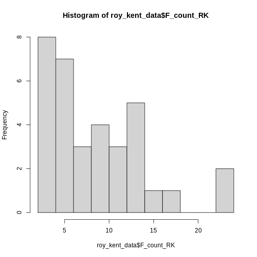This already provides us some more useful information. Roy seems to swear between 0 and 12 times most often and swears a lot in two episodes.

Let’s try increasing the number of breaks to 20.

R

hist(roy_kent_data$F_count_RK, breaks = 20)

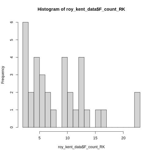
Here, an interesting pattern seems to emerge. Three different clusters of swear counts show up, one where Roy swears between 0 - 7 times, presumably because he has little screen-time in the episode. One cluster where Roy swears between 9-17 times, which more closely resembles his average swearing amount. And finally two episodes where Roy flies of the handle and swears a whopping max(roy_kent_data$F_count_RK) = 23 times!

In order to figure out what makes Roy swear so much, let’s plot the number of times Roy swears by episode!

ggplot2

For most of our plotting needs (except the beautiful hist()), we will make use of the package ggplot2 which is part of the larger collection of packages tidyverse and provides some really useful plotting functions. Most importantly, ggplot provides a useful grammar of plotting functions that always follow the same format.

You start out with the function ggplot() and give it our data, simple enough. Here, we start working with the entire dataframe, not just vectors. We can simply pass it into ggplot() and later on declare which variables we want to use.

R

ggplot(data = roy_kent_data)

ERROR

Error in ggplot(data = roy_kent_data): could not find function "ggplot"

Oops, R tells us that it cannot find this function. Most of the time, this is because you forgot to load the package beforehand. Let’s try again:

R

library(ggplot2)

ggplot(data = roy_kent_data)

Now it works, but not really. For now, this code only tells the function which data we are using, not what to do with it.

In order to actually see a plot, we need to provide information about the visual properties, the aesthetics that the plot should have. The mapping argument tells the function how the data relates to the visual properties of the plot. We define this mapping using the function aes(). Here, we declare the columns that we want on the x-axis and y-axis.

R

ggplot(
  data = roy_kent_data,
  mapping = aes(x = Episode_order, y = F_count_RK)
)

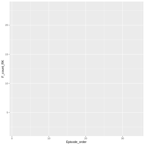
While we cannot see anything useful yet, we already notice some changes. The plot now correctly shows the names of the variables on the axes. Also, the ranges of numbers printed on the axes matches the minimum and maximum values.

Now that we provided the data and the mapping of variables to the plot, we can start building our proper visualization. This is done on top of the basics declared in ggplot(). This technique is called layering and it allows you to combine multiple new changes to a plot easily using a simple +. To add a plot showing the number of Fucks given by Roy during an episode, we can use geom_point().

R

ggplot(
  data = roy_kent_data,
  mapping = aes(x = Episode_order, y = F_count_RK)
) +
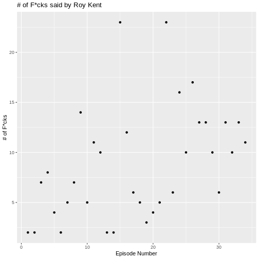
  geom_point()

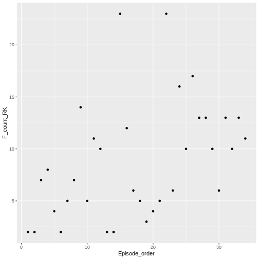
geom_point() adds a simple scatter-plot element to the graph.

We can change the labels to make the graph more polished using labs().

R

ggplot(
  data = roy_kent_data,
  mapping = aes(x = Episode_order, y = F_count_RK)
) +
  geom_point()+
  labs(
    title = "# of F*cks said by Roy Kent",
    x = "Episode Number",
    y = "# of F*cks"
  )

There seems to be a small trend showing that Roy swears more later in the series. We can visualize this trend by adding another layered visual geom_smooth().

R

ggplot(
  data = roy_kent_data,
  mapping = aes(x = Episode_order, y = F_count_RK)
) +
  geom_point()+
  labs(
    title = "# of F*cks said by Roy Kent",
    x = "Episode Number",
    y = "# of F*cks"
  )+
  geom_smooth(
    method = "lm", # this forces the trend-line to be linear
    se = FALSE
  )

OUTPUT

`geom_smooth()` using formula = 'y ~ x'

What might be causing this trend? Well, one possible candidate is that Roy goes from being a player on the team to being a coach on the team. This might cause him to yell at more people than usual. The variable that contains this information is Coaching_flag. Let’s learn something about it:

R

table(roy_kent_data$Coaching_flag)

OUTPUT


 No Yes
 14  20

It seems to have two values “Yes” and “No”, each being represented in the data more than 10 times.

We can also add this to our visualization from earlier, coloring in the dots by whether Roy was coaching or not. In order to do this, we need to add the color variable in the aesthetics mapping in the ggplot() function.

R

ggplot(
  data = roy_kent_data,
  mapping = aes(x = Episode_order, y = F_count_RK, color = Coaching_flag)
) +
  geom_point()+
  labs(
    title = "# of F*cks said by Roy Kent",
    x = "Episode Number",
    y = "# of F*cks"
  )+
  geom_smooth(
    method = "lm", # this forces the trend-line to be linear
    se = FALSE
  )

OUTPUT

`geom_smooth()` using formula = 'y ~ x'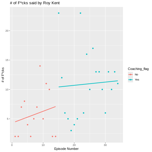

Now, a clearer picture emerges. Roy starts of pretty slow as a player, but then begins to swear a lot in the episodes that he is coaching in.

Making plots prettier using themes

The basic plots already look okay and are enough for just finding something out about data. But you can make them even more enticing by using a theme. Themes in ggplot are collections of visual settings that control the background of the plot, the text size of the axis and some other things.

I often use theme_classic() or theme_minimal(), but you can try out different themes or even write your own!

R

ggplot(
  data = roy_kent_data,
  mapping = aes(x = Episode_order, y = F_count_RK, color = Coaching_flag)
) +
  geom_point()+
  labs(
    title = "# of F*cks said by Roy Kent",
    x = "Episode Number",
    y = "# of F*cks"
  )+
  geom_smooth(
    method = "lm", # this forces the trend-line to be linear
    se = FALSE
  )+
  theme_minimal()

OUTPUT

`geom_smooth()` using formula = 'y ~ x'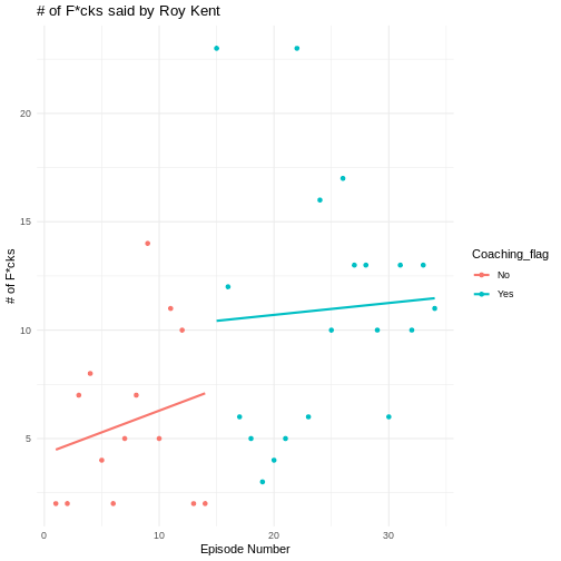

Challenges

Challenge 1

Figure out what information is stored in the column F_count_total. Compute the descriptive information (mean, standard deviation, minimum and maximum) for this variable.

Challenge 2

Compare the descriptive information to those for F_count_RK. Which one is bigger, why?

Compute the difference between the two variables. What does it represent. Compare the difference to F_count_RK. Which has the higher average value?

Show me the solution

R

f_count_others <- roy_kent_data$F_count_total - roy_kent_data$F_count_RK

mean(f_count_others)

OUTPUT

[1] 13

R

mean(roy_kent_data$F_count_RK)

OUTPUT

[1] 8.823529

Challenge 3

Plot a histogram of F_count_total. Try different values of breaks, which seems most interesting to you?

Challenge 4

Visualize the relationship between the amount of time Roy Kent said “Fuck” and the Imdb rating of that episode using geom_point().

Show me the solution

R

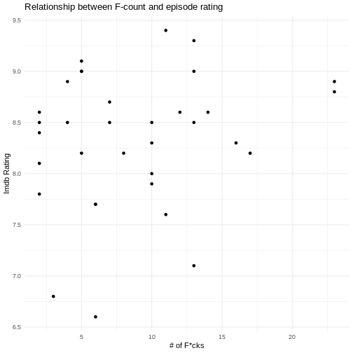
ggplot(
  data = roy_kent_data,
  mapping = aes(x = F_count_RK, y = Imdb_rating)
)+
  geom_point()+
  labs(
    title = "Relationship between F-count and episode rating",
    x = "# of F*cks",
    y = "Imdb Rating"
  )+
  theme_minimal()

Challenge 5

Be creative! What else can you notice in the data? Try to make an interesting plot.

Key Points

Get an overview of the data by inspecting it or using glimpse() / describe()
Consult a codebook for more in-depth descriptions of the variables in the data
Visualize the distribution of a variable using hist()
Use ggplot(data = data, mapping = aes()) to provide the data and mapping to the plots
Add visualization steps like geom_point() or geom_smooth() using +

Content from Data Visualization (2)

Last updated on 2025-06-24 | Edit this page

Overview

Questions

How can you visualize categorical data?
How to visualize the relationship of categorical and numerical data?

Objectives

Get to know the DASS data from Kaggle
Explain how to plot distribution of numerical data using geom_histogram() and geom_density()
Demonstrate how to group distributions by categorical variables

A new set of data

In this section, we will work with a new set of data. Download this data here and place it in your data folder. There is also a codebook available to download here.

The data originates from an online version of the Depression Anxiety Stress Scales (DASS), collected between 2017-2019 and retrieved from Kaggle. Participants took the test to receive personalized results and could opt into a research survey. The dataset includes responses to 42 DASS items (rated on a 4-point scale), response times, and question positions. Additional data includes:

Demographics (age, gender, education, native language, handedness, religion, sexual orientation, race, marital status, family size, major, country).
Big Five Personality Traits (via the Ten Item Personality Inventory - TIPI).
Vocabulary Check (includes fake words for validity checks).

Let’s read in the data first. In my case, it is placed inside a subfolder of data/ called kaggle_dass/. You may need to adjust the path on your end.

R

dass_data <- read.csv("data/kaggle_dass/data.csv")

As you might already see, this data is quite large. In the Environment tab we can see that it contains almost 40.000 entries and 172 variables. For now, we will be working with some of the demographic statistics. We will delve into the actual score in a later episode. You can find information on this data in the codebook provided here.

Read this codebook in order to familiarize yourself with the data. Then inspect it visually by clicking on the frame or running View(dass_data). What do you notice?

First, let’s start getting an overview of the demographics of test-takers. What is their gender, age and education? Compute descriptive statistics for age and inspect gender and education using table()

R

table(dass_data$gender)

OUTPUT


    0     1     2     3
   67  8789 30367   552

R

mean(dass_data$age)

OUTPUT

[1] 23.61217

R

sd(dass_data$age)

OUTPUT

[1] 21.58172

R

range(dass_data$age) # This outputs min() and max() at the same time

OUTPUT

[1]   13 1998

R

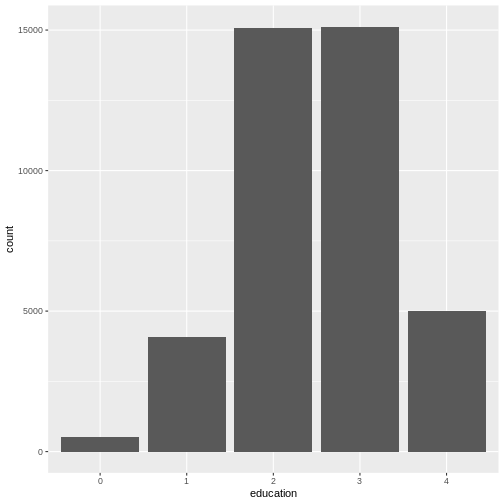
table(dass_data$education)

OUTPUT


    0     1     2     3     4
  515  4066 15066 15120  5008

The maximum value of age seems a bit implausible, unless Elrond has decided to take the DASS after Galadriel started flirting with Sauron (sorry, Annatar) again.

Histograms

We can get an overview of age by using our trust hist():

R

hist(dass_data$age)

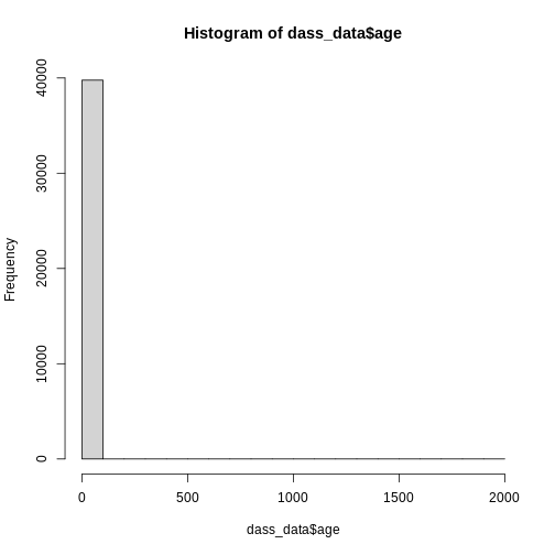
However, this graph is heavily skewed by the outliers in age. We can address this issue easily by converting to a ggplot histogram. The xlim() layer can restrict the values that are displayed in the plot and gives us a warning about how many values were discarded.

R

library(ggplot2) # Don't forget to load the package

ggplot(
  data = dass_data,
  mapping = aes(x = age)
)+
  geom_histogram()+
  xlim(0, 100)

OUTPUT

`stat_bin()` using `bins = 30`. Pick better value with `binwidth`.

WARNING

Warning: Removed 7 rows containing non-finite outside the scale range
(`stat_bin()`).

WARNING

Warning: Removed 2 rows containing missing values or values outside the scale range
(`geom_bar()`).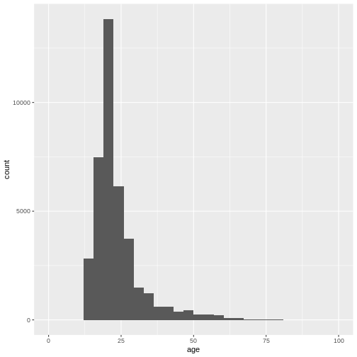

Again, the number of bins might be a bit small:

R

ggplot(
  data = dass_data,
  mapping = aes(x = age)
)+
  geom_histogram(bins = 100)+
  xlim(0, 100)

WARNING

Warning: Removed 7 rows containing non-finite outside the scale range
(`stat_bin()`).

WARNING

Warning: Removed 2 rows containing missing values or values outside the scale range
(`geom_bar()`).

We can also adjust the size of the bins, not the number of bins by using the binwidth argument.

R

ggplot(
  data = dass_data,
  mapping = aes(x = age)
)+
  geom_histogram(binwidth = 1)+
  xlim(0, 100)

WARNING

Warning: Removed 7 rows containing non-finite outside the scale range
(`stat_bin()`).

WARNING

Warning: Removed 2 rows containing missing values or values outside the scale range
(`geom_bar()`).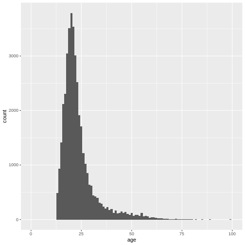

This gives us a nice overview of the distribution of each possible distinct age. It seems to peak around 23 and then slowly decline in frequency. This is in line with what you would expect from data from a free online personality questionnaire.

Density plots

Often, what interests us is not the number of occurrences for a given value, but rather which values are common and which values are uncommon. By dividing the number of occurrences for a given value by the total number of observation, we can obtain a density-plot. In ggplot you achieve this by using geom_density() instead of geom_histogram().

R

ggplot(
  data = dass_data,
  mapping = aes(x = age)
)+
  geom_density()+
  xlim(0, 100)

WARNING

Warning: Removed 7 rows containing non-finite outside the scale range
(`stat_density()`).

This describes the overall age distribution, but we can also look at the age distribution by education status. What would you expect?

Again, we do this by using the color argument in aes(), as I want different colored density plots for each education level.

R

ggplot(
  data = dass_data,
  mapping = aes(x = age, color = education)
)+
  geom_density()+
  xlim(0, 100)

WARNING

Warning: Removed 7 rows containing non-finite outside the scale range
(`stat_density()`).

WARNING

Warning: The following aesthetics were dropped during statistical transformation:
colour.
ℹ This can happen when ggplot fails to infer the correct grouping structure in
  the data.
ℹ Did you forget to specify a `group` aesthetic or to convert a numerical
  variable into a factor?

It seems like this didn’t work. And the warning message tells us why. We forgot to specify a group variable that tells the plotting function that we not only want different colors, we also want different lines, grouped by education status:

R

ggplot(
  data = dass_data,
  mapping = aes(x = age, color = education, group = education)
)+
  geom_density()+
  xlim(0, 100)

WARNING

Warning: Removed 7 rows containing non-finite outside the scale range
(`stat_density()`).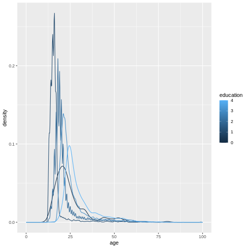

Because education is a numerical variable, ggplot uses a sliding color scale to color its values. I think it looks a little more beautiful if we declare that despite having numbers as entries, education is not strictly numerical. The different numbers represent distinct levels of educational attainment. We can encode this using factor() to convert education into a variable-type called factor that has this property.

R

dass_data$education <- factor(dass_data$education)
ggplot(
  data = dass_data,
  mapping = aes(x = age, color = education, group = education)
)+
  geom_density()+
  xlim(0, 100)

WARNING

Warning: Removed 7 rows containing non-finite outside the scale range
(`stat_density()`).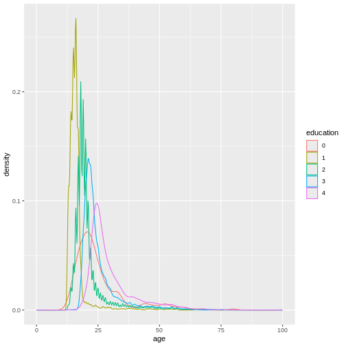

We can make this graph look a little bit better by filling in the area under the curves with the color aswell and making them slightly transparent. This can be done using the fill argument and the alpha argument. Let’s also give the graph a proper title and labels.

R

ggplot(
  data = dass_data,
  mapping = aes(x = age, color = education, group = education, fill = education)
)+
  geom_density(alpha = 0.5)+
  xlim(0, 100)+
  labs(
    title = "Age distribution by education status",
    x = "Age",
    y = "Density"
  ) +
  theme_minimal()

WARNING

Warning: Removed 7 rows containing non-finite outside the scale range
(`stat_density()`).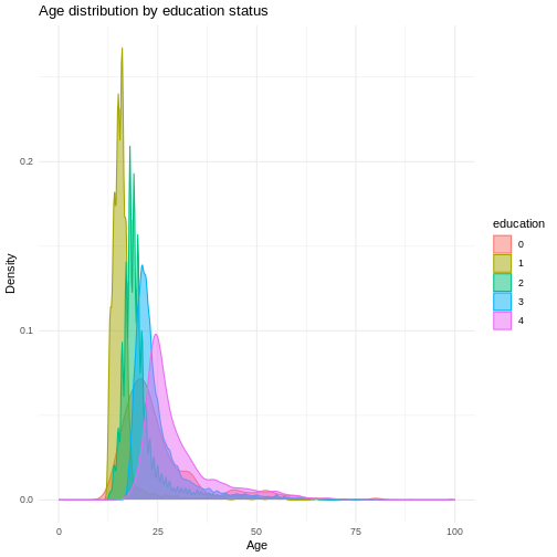

In this graph, we can see exactly what we would expect. As the highest achieved education increases, the age of test-takers generally gets larger as-well. There just are very little people under 20 with a PhD.

Bar Charts

As a last step of exploration, let’s visualize the number of people that achieved a certain educational status. A bar chart is perfect for this:

R

ggplot(
  data = dass_data,
  mapping = aes(x = education)
)+
  geom_bar()

This visualizes the same numbers as table(dass_data$education) and sometimes, you may not need to create a plot if the numbers already tell you everything you need to know. However, remember that often you need to communicate your results to other people. And as they say “A picture says more than 1000 words”.

We can also include gender as a variable here, in order to compare educational attainment between available genders. Let’s plot gender on the x-axis and color the different education levels.

R

ggplot(
  data = dass_data,
  mapping = aes(x = gender, fill = education)
)+
  geom_bar()

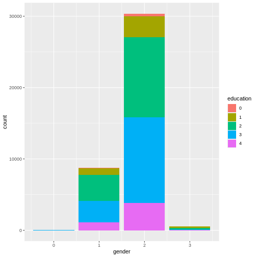
This graph is very good at showing one thing: there are more females in the data than males. However, this is not the comparison we are interested in. We can plot relative frequencies of education by gender by using the argument position = "fill".

R

ggplot(
  data = dass_data,
  mapping = aes(x = gender, fill = education)
)+
  geom_bar(position = "fill")

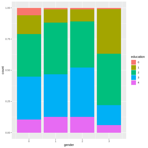
This plot shows that education levels don’t differ dramatically between males and females in our sample, with females holding a university degree more often than males.

Common Problems

This section is lifted from R for Data Science (2e).

As you start to run R code, you’re likely to run into problems. Don’t worry — it happens to everyone. We have all been writing R code for years, but every day we still write code that doesn’t work on the first try!

Start by carefully comparing the code that you’re running to the code in the book. R is extremely picky, and a misplaced character can make all the difference. Make sure that every ( is matched with a ) and every " is paired with another ". Sometimes you’ll run the code and nothing happens. Check the left-hand of your console: if it’s a +, it means that R doesn’t think you’ve typed a complete expression and it’s waiting for you to finish it. In this case, it’s usually easy to start from scratch again by pressing ESCAPE to abort processing the current command.

One common problem when creating ggplot2 graphics is to put the + in the wrong place: it has to come at the end of the line, not the start. In other words, make sure you haven’t accidentally written code like this:

R

ggplot(data = mpg) 
+ geom_point(mapping = aes(x = displ, y = hwy))

If you’re still stuck, try the help. You can get help about any R function by running ?function_name in the console, or highlighting the function name and pressing F1 in RStudio. Don’t worry if the help doesn’t seem that helpful - instead skip down to the examples and look for code that matches what you’re trying to do.

If that doesn’t help, carefully read the error message. Sometimes the answer will be buried there! But when you’re new to R, even if the answer is in the error message, you might not yet know how to understand it. Another great tool is Google: try googling the error message, as it’s likely someone else has had the same problem, and has gotten help online.

Recap - Knowing your data!

It’s important to understand your data, its sources and quirks before you start working with it! This is why the last few episodes focused so much on descriptive statistics and plots. Get to know the structure of your data, figure out where it came from and what type of people constitute the sample. Monitor your key variables for implausible or impossible values. Statistical outliers we can define later, but make sure to identify issues with impossible values early on!

Challenges

Challenge 1

Review what we learned about the DASS data so far. What are the key demographic indicators? Is there anything else important to note?

Challenge 2

Read the codebook. What is the difference between Q1A, Q1E and Q1I?

Challenge 3

Provide descriptive statistics of the time it took participants to complete the DASS-part of the survey. What variable is this stored in? What is the average time? Are there any outliers? What is the average time without outliers?

Challenge 4

Plot a distribution of the elapsed test time. What might be a sensible cutoff for outliers?

Plot a distribution of elapsed test time by whether English was the native language. What do you expect? What can you see? What are your thoughts on the distribution?

Show me the solution

R

dass_data$engnat <- factor(dass_data$engnat)

ggplot(
  data = dass_data,
  mapping = aes(
    x = testelapse, fill = engnat, group = engnat
  )
)+
  geom_density(alpha = 0.5)+
  xlim(0, 3000)+
  labs(
    title = "Distribution of test completion times",
    subtitle = "By Mother Tongue",
    x = "Test completion time (s)",
    y = "Density"
  )+
  theme_minimal()

WARNING

Warning: Removed 399 rows containing non-finite outside the scale range
(`stat_density()`).

Challenge 5

Learn something about the handedness of test-takers. Get the number of test-takers with each handedness using table and visualize it using geom_bar().

Plot the handedness of test-takers by educational status. Do you see any differences?

Show me the solution

R

ggplot(
  data = dass_data,
  mapping = aes(
    x = hand,
    fill = education,
    group = education
  )
)+
  geom_bar(position = "fill")+
  labs(
    title = "Educational attainment by handedness",
    x = "Handedness (0 = NA, 1 = Right, 2 = Left, 3 = Both)",
    y = "Proportion"
  )+
  theme_minimal()

Key Points

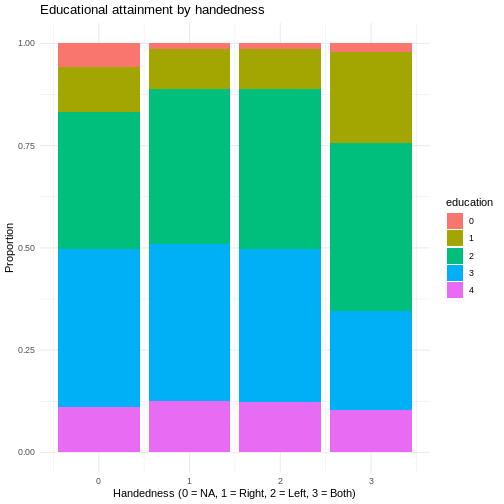
Get to know new data by inspecting it and computing key descriptive statistics
Visualize distributions of key variables in order to learn about factors that impact them
Visualize distribution of a numeric and a categorical variable using geom_density()
Visualize distribution of two categorial variables using geom_bar()

Content from Filtering data

Last updated on 2025-06-24 | Edit this page

Overview

Questions

How do you filter invalid data?
How do you chain commands using the pipe %>%?
How can I select only some columns of my data?

Objectives

Explain how to filter rows using filter()
Demonstrate how to select columns using select()
Explain how to use the pipe %>% to facilitate clean code

Filtering

In the earlier episodes, we have already seen some impossible values in age and testelapse. In our analyses, we probably want to exclude those values, or at the very least investigate what is wrong. In order to do that, we need to filter our data - to make sure it only has those observations that we actually want. The dplyr package provides a useful function for this: filter().

Let’s start by again loading in our data, and also loading the package dplyr.

R

library(dplyr)

OUTPUT


Attaching package: 'dplyr'

OUTPUT

The following objects are masked from 'package:stats':

    filter, lag

OUTPUT

The following objects are masked from 'package:base':

    intersect, setdiff, setequal, union

R

dass_data <- read.csv("data/kaggle_dass/data.csv")

The filter function works with two key inputs, the data and the arguments that you want to filter by. The data is always the first argument in the filter function. The following arguments are the filter conditions. For example, in order to only include people that are 20 years old, we can run the following code:

R

twenty_year_olds <- filter(dass_data, age == 20)
# Lets make sure this worked
table(twenty_year_olds$age)

OUTPUT


  20
3789

R

# range(twenty_year_olds$age) # OR THIS
# unique(twenty_year_olds$age) # OR THIS
# OR other things that come to mind can check this

Now, in order to only include participants aged between 0 and 100, which seems like a reasonable range, we can condition on age >= 0 & age <= 100.

R

valid_age_dass <- filter(dass_data, age >= 0 & age <= 100)

Let’s check if this worked using a histogram.

R

hist(valid_age_dass$age, breaks = 50)

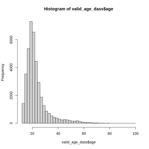
Looks good! Now it is always a good idea to inspect the values you removed from the data, in order to make sure that you did not remove something you intended to keep, and to learn something about the data you removed.

Let’s first check how many rows of data we actually removed:

R

n_rows_original <- nrow(dass_data)

n_rows_valid_age <- nrow(valid_age_dass)

n_rows_removed <- n_rows_original - n_rows_valid_age

n_rows_removed

OUTPUT

[1] 7

This seems okay! Only 7 removed cases out of almost 40000 entries is negligible. Nonentheless, let’s investigate this further.

R

impossible_age_data <- filter(dass_data, age < 0 | age > 100)

Now we have a dataset that contains only the few cases with invalid ages. We can just look at the ages first:

R

impossible_age_data$age

OUTPUT

[1]  223 1996  117 1998  115 1993 1991

Now, let’s try investigating the a little deeper. Do the people with invalid entries in age have valid entries in the other columns? Try to figure this out by visually inspecting the data. Where are they from? Do the responses to other questions seem odd?

This is possible, but somewhat hard to do for data with 170 columns. Looking through all of them might make you a bit tired after the third investigation of invalid data. What we really need is to look at only a few columns that interest us.

Selecting columns

This is where the function select() comes in. It enables us to only retain some columns from a dataset for further analysis. You just give it the data as the first argument and then list all of the columns you want to keep.

R

inspection_data_impossible_age <- select(
    impossible_age_data,
    age, country, engnat, testelapse
  )

inspection_data_impossible_age

OUTPUT

   age country engnat testelapse
1  223      MY      2        456
2 1996      MY      2        259
3  117      US      1        114
4 1998      MY      2        196
5  115      AR      2        238
6 1993      MY      2        232
7 1991      MY      2        240

Here, we can see that our original data is reduced to the four columns we specified above age, country, engnat, testelapse. Do any of them look strange? What happened in the age column?

To me, none of the other entries seem strange, the time it took them to complete the survey is plausible, they don’t show a clear trend of being from the same country. It seems that some people mistook the age question and entered their year of birth instead. Later on, we can try to fix this.

But before we do that, there are some more things about select() that we can learn. It is one of the most useful functions in my daily life, as it allows me to keep only those columns that I am actually interested in. And it has many more features than just listing the columns!

For example, note that the last few columns of the data are all the demographic information. This is starting with education and ending with major.

To select everything from education to major:

R

# colnames() gives us the names of the columns only
colnames(select(valid_age_dass, education:major))

OUTPUT

 [1] "education"             "urban"                 "gender"
 [4] "engnat"                "age"                   "screensize"
 [7] "uniquenetworklocation" "hand"                  "religion"
[10] "orientation"           "race"                  "voted"
[13] "married"               "familysize"            "major"

We can also select all character columns using where():

R

colnames(select(valid_age_dass, where(is.character)))

OUTPUT

[1] "country" "major"

Or we can select all columns that start with the letter “Q”:

R

colnames(select(valid_age_dass, starts_with("Q")))

OUTPUT

  [1] "Q1A"  "Q1I"  "Q1E"  "Q2A"  "Q2I"  "Q2E"  "Q3A"  "Q3I"  "Q3E"  "Q4A"
 [11] "Q4I"  "Q4E"  "Q5A"  "Q5I"  "Q5E"  "Q6A"  "Q6I"  "Q6E"  "Q7A"  "Q7I"
 [21] "Q7E"  "Q8A"  "Q8I"  "Q8E"  "Q9A"  "Q9I"  "Q9E"  "Q10A" "Q10I" "Q10E"
 [31] "Q11A" "Q11I" "Q11E" "Q12A" "Q12I" "Q12E" "Q13A" "Q13I" "Q13E" "Q14A"
 [41] "Q14I" "Q14E" "Q15A" "Q15I" "Q15E" "Q16A" "Q16I" "Q16E" "Q17A" "Q17I"
 [51] "Q17E" "Q18A" "Q18I" "Q18E" "Q19A" "Q19I" "Q19E" "Q20A" "Q20I" "Q20E"
 [61] "Q21A" "Q21I" "Q21E" "Q22A" "Q22I" "Q22E" "Q23A" "Q23I" "Q23E" "Q24A"
 [71] "Q24I" "Q24E" "Q25A" "Q25I" "Q25E" "Q26A" "Q26I" "Q26E" "Q27A" "Q27I"
 [81] "Q27E" "Q28A" "Q28I" "Q28E" "Q29A" "Q29I" "Q29E" "Q30A" "Q30I" "Q30E"
 [91] "Q31A" "Q31I" "Q31E" "Q32A" "Q32I" "Q32E" "Q33A" "Q33I" "Q33E" "Q34A"
[101] "Q34I" "Q34E" "Q35A" "Q35I" "Q35E" "Q36A" "Q36I" "Q36E" "Q37A" "Q37I"
[111] "Q37E" "Q38A" "Q38I" "Q38E" "Q39A" "Q39I" "Q39E" "Q40A" "Q40I" "Q40E"
[121] "Q41A" "Q41I" "Q41E" "Q42A" "Q42I" "Q42E"

There are a number of helper functions you can use within select():

starts_with("abc"): matches names that begin with “abc”.
ends_with("xyz"): matches names that end with “xyz”.
contains("ijk"): matches names that contain “ijk”.
num_range("x", 1:3): matches x1, x2 and x3.

You can also remove columns using select by simply negating the argument using !:

R

colnames(select(valid_age_dass, !starts_with("Q")))

OUTPUT

 [1] "country"               "source"                "introelapse"
 [4] "testelapse"            "surveyelapse"          "TIPI1"
 [7] "TIPI2"                 "TIPI3"                 "TIPI4"
[10] "TIPI5"                 "TIPI6"                 "TIPI7"
[13] "TIPI8"                 "TIPI9"                 "TIPI10"
[16] "VCL1"                  "VCL2"                  "VCL3"
[19] "VCL4"                  "VCL5"                  "VCL6"
[22] "VCL7"                  "VCL8"                  "VCL9"
[25] "VCL10"                 "VCL11"                 "VCL12"
[28] "VCL13"                 "VCL14"                 "VCL15"
[31] "VCL16"                 "education"             "urban"
[34] "gender"                "engnat"                "age"
[37] "screensize"            "uniquenetworklocation" "hand"
[40] "religion"              "orientation"           "race"
[43] "voted"                 "married"               "familysize"
[46] "major"

Now we will only get those columns that don’t start with “Q”.

Selecting a column twice

You can also use select to reorder the columns in your dataset. For example, notice that the following two bits of code return differently order data:

R

# head() gives us the first 10 values only
head(select(valid_age_dass, age, country, testelapse), 10)

OUTPUT

   age country testelapse
1   16      IN        167
2   16      US        193
3   17      PL        271
4   13      US        261
5   19      MY        164
6   20      US        349
7   17      MX      45459
8   29      GB        232
9   16      US        195
10  18      DE        120

R

head(select(valid_age_dass, testelapse, age, country), 10)

OUTPUT

   testelapse age country
1         167  16      IN
2         193  16      US
3         271  17      PL
4         261  13      US
5         164  19      MY
6         349  20      US
7       45459  17      MX
8         232  29      GB
9         195  16      US
10        120  18      DE

Using the function everything(), you can select all columns.

What happens, when you select a column twice? Try running the following examples, what do you notice about the position of columns?

R

select(valid_age_dass, age, country, age)

select(valid_age_dass, age, country, everything())

Using the pipe `%>%`

Let’s retrace some of the steps that we took. We had the original data dass_data and then filtered out those rows with invalid entries in age. Then, we tried selecting only a couple of columns in order to make the data more manageable. In code:

R

impossible_age_data <- filter(dass_data, age < 0 | age > 100)

inspection_data_impossible_age <- select(
  impossible_age_data,
  age, country, engnat, testelapse
  )

Notice how the first argument for both the filter() and the select() function is always the data. This is also true for the ggplot() function. And it’s no coincidence! In R, there exists a special symbol, called the pipe %>%, that has the following property: It takes the output of the previous function and uses it as the first input in the following function.

This can make our example considerably easier to type:

R

dass_data %>% 
  filter(age < 0 | age > 100) %>% 
  select(age, country, engnat, testelapse)

OUTPUT

   age country engnat testelapse
1  223      MY      2        456
2 1996      MY      2        259
3  117      US      1        114
4 1998      MY      2        196
5  115      AR      2        238
6 1993      MY      2        232
7 1991      MY      2        240

Notice how the pipe is always written at the end of a line. This makes it easier to understand and to read. As we go to the next line, whatever is outputted is used as input in the following line. So the original data dass_data is used as the first input in the filter function, and the filtered data is used as the first input in the select function.

To use the pipe, you can either type it out yourself or use the Keyboard-Shortcut Ctrl + Shift + M.

Plotting using the pipe

We have seen that the pipe %>% allows us to chain multiple functions together, making our code cleaner and easier to read. This can be particularly useful when working with ggplot2, where we often build plots step by step. Since ggplot() takes the data as its first argument, we can use the pipe to make our code more readable.

For example, let’s say we want to create a histogram of valid ages in our dataset. Instead of writing:

R

library(ggplot2)

ggplot(valid_age_dass, aes(x = age)) +
  geom_histogram(bins = 50)

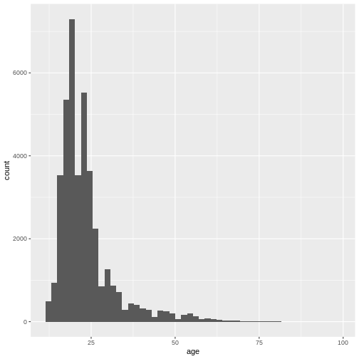
We can write:

R

valid_age_dass %>%
  ggplot(aes(x = age)) +
  geom_histogram(bins = 50)

This makes it clear that valid_age_dass is the dataset being used, and it improves readability.

Using the pipe for the second argument

By default, the pipe places the output of the previous code as the first argument in the following function. In most cases, this is exactly what we want to have. If you want to be more explicit about where the pipe should place the output, you can do this by placing a . as the placeholder for piped-data.

R

n_bins <- 30

n_bins %>%
  hist(valid_age_dass$age, .)

Numbered vs. Named Arguments

The pipe is made possible because most functions in the packages included in tidyverse, like dplyr and ggplot have the data as their first argument. This makes it simple to pipe-through results from one function to the next, without having to explicitly type function(data = something) every time. In principle, almost all functions have a natural order in which they expect arguments to occur. For example: ggplot() expects data as the first argument and information about the mapping as the second argument. This is why we always typed:

R

ggplot(
  data = valid_age_dass,
  mapping = aes(x = age)
)+
  geom_density()

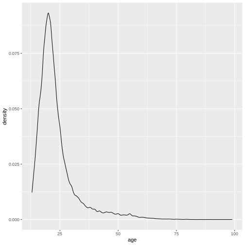
Notice that if we don’t specify the argument names, we still receive the same results. The function just uses the inputs you give it to match the arguments in the order in which they occur.

R

ggplot(
  valid_age_dass, # Now it just automatically thinks this is data = 
  aes(x = age) # and this is mapping = 
)+
  geom_density()

This is what makes this possible:

R

valid_age_dass %>%
  ggplot(aes(x = age)) +
  geom_density()

However, if we try to supply an argument in a place where it doesn’t belong, we get an error:

R

n_bins = 50 
valid_age_dass %>%
  ggplot(aes(x = age)) +
  geom_histogram(n_bins)  # This will cause an error!

ERROR

Error in `geom_histogram()`:
! `mapping` must be created by `aes()`.

geom_histogram does not expect the number of bins to be the first argument, but rather the mapping! Therefore, we need to declare this properly:

R

valid_age_dass %>%
  ggplot(aes(x = age)) +
  geom_histogram(bins = n_bins)

To learn about the order of arguments of a function, use ?function and inspect the help file.

Common Problems

Using one pipe too little

A common mistake is forgetting to use a pipe between arguments of a chain. For example:

R

valid_age_dass %>% 
  filter(age > 18)
  select(age, country)

Here, select() is not part of the pipeline because the pipe is missing after filter(age > 18). This can lead to unexpected errors or incorrect results. The correct way to write this is:

R

valid_age_dass %>% 
  filter(age > 18) %>% 
  select(age, country)

Using one pipe too much

Another common problem is using one pipe too many without having a function following it.

R

valid_age_dass %>% 
  filter(age > 18) %>% 
  select(age, country) %>%

ERROR

Error in parse(text = input): <text>:4:0: unexpected end of input
2:   filter(age > 18) %>%
3:   select(age, country) %>%
  ^

This can cause some really strange errors that never say anything about the pipe being superfluous. Make sure that all your pipe “lead somewhere”.

Using a pipe instead of `+` for `ggplot()`

A source of confusion stems from the difference between the pipe %>% and ggplot2’s +. They both serve very similar purposes, namely adding together a chain of functions. However, make sure you use %>% for everything except ggplot-functions. Here, you will also receive an error that is a little more informative:

R

valid_age_dass %>% 
  ggplot(aes(x = age)) %>% 
  geom_density()

ERROR

Error in `geom_density()` at magrittr/R/pipe.R:136:3:
! `mapping` must be created by `aes()`.
ℹ Did you use `%>%` or `|>` instead of `+`?

Using `=` Instead of `==` in `filter()`

Another common error is using = instead of == when filtering data. For example:

R

valid_age_dass %>% 
  filter(country = "US") %>%  # Incorrect!
  head()

ERROR

Error in `filter()`:
! We detected a named input.
ℹ This usually means that you've used `=` instead of `==`.
ℹ Did you mean `country == "US"`?

This will result in an error because = is used for assigning values, while == is used for comparisons. The correct syntax is:

R

valid_age_dass %>% 
  filter(country == "US") %>% 
  select(country, engnat, education) %>% 
  head()

OUTPUT

  country engnat education
1      US      1         2
2      US      1         1
3      US      2         2
4      US      2         2
5      US      1         1
6      US      1         2

Challenges

Challenge 1

Filter the complete dass_data. Create one dataset containing only entries with people from the United States and one dataset containing only entries from Great Britain. Compare the number of entries in each dataset. What percentage of the total submissions came from these two countries?

What is the average age of participants from the two countries?

Challenge 2

Create a filtered dataset based on the following conditions:

The participant took less than 30 minutes to complete the DASS-part of the survey
English is the native language of the participant
There is an entry in the field major

Challenge 3

What arguments does the cut() function take? Make a list of the arguments and the order in which they have to be provided to the function.

Challenge 4

In a single chain of functions, create a dataset is filtered with the same conditions as above and contains only the following variables:

all demographic information, country information and the duration of the tests
all the answers to the DASS (and only the answers, not the position or timing)

Show me the solution

R

english_unversity_dass <- dass_data %>% 
  filter(testelapse < 1800) %>% 
  filter(engnat == 1) %>% 
  filter(major != "") %>% 
  select(starts_with("Q") & ends_with("A"), contains("elapse"), country, education:major)

write.csv(english_unversity_dass, "data/english_university_dass_data.csv")

Challenge 5

Save that dataset to a file english_university_dass_data.csv in your processed_data folder. You may need to use Google to find a function that you can use to save data.

Key Points

Use the pipe operator %>% to link multiple functions together
Use filter() to filter rows based on certain conditions
Use select() to keep only those rows that interest you

Content from Creating new columns

Last updated on 2025-06-24 | Edit this page

Overview

Questions

What function is used to create new columns in a dataset?
How can you generate a unique ID column for each row?
How can you modify an existing column?
How can you compute an average value over many columns in your data?

Objectives

Understand how to use mutate() to create new columns.
Learn how to add constant values, computed values, and conditionally assigned values to new columns.
Use ifelse() to create categorical columns based on conditions.
Learn efficient methods for computing row-wise sums and averages using rowSums() and rowMeans().
Understand the difference between sum() and rowSums() for column-wise and row-wise operations.

Making new columns

So far we have dealt with existing columns and worked on them. We have computed descriptive statistics, plotted basic overviews of data and cut the data just the way we like it using filter() and select(). Now, we will unlock a new power… the power of creation! Muhahahahaha.

Well, actually it’s just adding new columns to the dataset, but that’s still cool! Let’s start by reading in our DASS data again and loading the package dplyr.

R

library(dplyr)

OUTPUT


Attaching package: 'dplyr'

OUTPUT

The following objects are masked from 'package:stats':

    filter, lag

OUTPUT

The following objects are masked from 'package:base':

    intersect, setdiff, setequal, union

R

dass_data <- read.csv("data/kaggle_dass/data.csv")

To add a new column, we need the dplyr function mutate(). It changes - or mutates - columns in the dataset, like adding entirely new ones. The syntax is quite simple. The first argument is the data, allowing easy use of pipes, and the second argument is the code for the new column you want to have.

For example, if we want to create a new column that carries just a single value, we type the following:

R

dass_data <- dass_data %>% 
  mutate(single_value_column = 42)

To check if this worked:

R

unique(dass_data$single_value_column)

OUTPUT

[1] 42

Saving progress

Notice how we had to assign the dataset to itself in order to save the progress we have made. If you do not do this, and just write down the pipeline, the end result will be outputted to the console, not stored in an object that we can use later.

R

dass_data %>% 
  head(6) %>% 
  mutate(some_column = "I have a value!") %>% 
  select(country, some_column)

OUTPUT

  country     some_column
1      IN I have a value!
2      US I have a value!
3      PL I have a value!
4      US I have a value!
5      MY I have a value!
6      US I have a value!

You can easily assign the new data to something with the same name, overriding the previous status. But be careful with this, I recommend you use new names for the data after filtering, selecting, and mutating existing columns. These operations change the original data (they remove some information) and should thus be stored in a new object, like filtered_dass_data.

We can do much more interesting things than just placing a constant in the new column. For example, we can use row_number() to create a running number of entries in our data - an id of sort.

R

dass_data <- dass_data %>% 
  mutate(entry_id = row_number())

dass_data %>% 
  select(country, testelapse, entry_id) %>% 
  head()

OUTPUT

  country testelapse entry_id
1      IN        167        1
2      US        193        2
3      PL        271        3
4      US        261        4
5      MY        164        5
6      US        349        6

Mutating existing columns

We can also base our mutation on existing columns. testelapse is in seconds right now, let’s add a new column that is the elapsed test time in minutes.

R

dass_data <- dass_data %>% 
  mutate(
    testelapse_min = testelapse / 60
  )

mean(dass_data$testelapse)

OUTPUT

[1] 2684.843

R

mean(dass_data$testelapse_min)

OUTPUT

[1] 44.74738

Another function I often use when creating new columns is ifelse(). It works using three arguments.

R

a = 5
b = 3

ifelse(
  a > b, # The condition
  "a is greater", # IF yes
  "a is smaller" # IF no
)

OUTPUT

[1] "a is greater"

We can use this to make a new column that tells us whether an entry came from the United States.

R

dass_data <- dass_data %>% 
  mutate(is_from_us = ifelse(country == "US", "yes", "no"))

table(dass_data$is_from_us)

OUTPUT


   no   yes
31566  8207

Adding existing columns

One of the most important uses of mutate() is adding together multiple columns. In our data, we have three columns indicating the length of elapsed time during survey completion, introelapse, testelapse and surveyelapse.

We can compute the sum of these three columns to get the total amount of elapsed time.

R

dass_data <- dass_data %>%
  mutate(
    total_elapse_seconds = introelapse + testelapse + surveyelapse
  )

Hint: Conduct Sanity Checks

When programming, you will make mistakes. There just is not a way around it. The only way to deal with it is trying to catch your mistakes as early as possible. Sometimes the computer will help you out by issuing an error or a warning. Sometimes it does not, because the code you wrote is technically valid but still does not exactly do what you want it to.

Therefore, it is important to conduct sanity checks! Try looking at the data and figure out if what you just did makes sense. In our case, let’s inspect the new column:

R

dass_data %>% 
  select(introelapse, testelapse, surveyelapse, total_elapse_seconds) %>% 
  head()

OUTPUT

  introelapse testelapse surveyelapse total_elapse_seconds
1          19        167          166                  352
2           1        193          186                  380
3           5        271          122                  398
4           3        261          336                  600
5        1766        164          157                 2087
6           4        349          213                  566

This looks good so far!

Now, this approach works well for a few columns, but gets tedious quickly when attempting to compute the sum or average over multiple columns. For this there exists a special fuction called rowSums(). This function takes a dataset, and computes the sums across all columns.

R

example_data <- data.frame(
  x = 1:4,
  y = 2:5,
  z = 3:6
)
example_data$sum <- rowSums(example_data)

example_data

OUTPUT

  x y z sum
1 1 2 3   6
2 2 3 4   9
3 3 4 5  12
4 4 5 6  15

However, in our case we do not want a sum across all columns of our data, but just some of the columns! To do this, we need to use across() inside the rowSums function to select specific columns.

R

dass_data %>%
  mutate(elapse_sum = rowSums(across(c("introelapse", "testelapse", "surveyelapse")))) %>% 
  select(introelapse, testelapse, surveyelapse, elapse_sum) %>% 
  head()

OUTPUT

  introelapse testelapse surveyelapse elapse_sum
1          19        167          166        352
2           1        193          186        380
3           5        271          122        398
4           3        261          336        600
5        1766        164          157       2087
6           4        349          213        566

Because across() also accepts the same input as select() we can use the special functions like starts_with(), ends_with() or contains().

R

dass_data %>%
  mutate(elapse_sum = rowSums(across(ends_with("elapse")))) %>% 
  select(ends_with("elapse"), elapse_sum) %>% 
  head()

OUTPUT

  introelapse testelapse surveyelapse elapse_sum
1          19        167          166        352
2           1        193          186        380
3           5        271          122        398
4           3        261          336        600
5        1766        164          157       2087
6           4        349          213        566

Similarly, we can use rowMeans() to compute the average test duration. The beautiful thing about mutate() is, that we can create multiple columns in one function call!

R

dass_data %>%
  mutate(
    constant_value = "I am a value!",
    id = row_number(),
    elapse_sum = rowSums(across(ends_with("elapse"))),
    elapse_mean = rowMeans(across(ends_with("elapse")))
  ) %>% 
  select(id, constant_value, ends_with("elapse"), elapse_sum, elapse_mean) %>% 
  head()

OUTPUT

  id constant_value introelapse testelapse surveyelapse elapse_sum elapse_mean
1  1  I am a value!          19        167          166        352    117.3333
2  2  I am a value!           1        193          186        380    126.6667
3  3  I am a value!           5        271          122        398    132.6667
4  4  I am a value!           3        261          336        600    200.0000
5  5  I am a value!        1766        164          157       2087    695.6667
6  6  I am a value!           4        349          213        566    188.6667

Pro Tip: mutate() + across()

Sometimes, you want to mutate multiple columns at once, applying the same function to all of them. For example, when you want to recode some values across all columns that share the incorrect format. Here, you can use mutate() in combination with across() to apply a function to all of them. In our case, lets compute the elapse time in minutes for all elapse columns.

R

dass_data %>% 
  mutate(
    across(
      ends_with("elapse"), # Select the columns you want
      ~ .x / 60, # Write the function to apply to all of them
      # Use this special function syntax ~ and a .x as the argument to be filled
      .names = "{.col}_minutes" # Give out new names by using the old name
      # which will take the place of {.col} and some new value.
    )
  ) %>% 
  select(contains("elapse")) %>% 
  head()

OUTPUT

  introelapse testelapse surveyelapse testelapse_min total_elapse_seconds
1          19        167          166       2.783333                  352
2           1        193          186       3.216667                  380
3           5        271          122       4.516667                  398
4           3        261          336       4.350000                  600
5        1766        164          157       2.733333                 2087
6           4        349          213       5.816667                  566
  introelapse_minutes testelapse_minutes surveyelapse_minutes
1          0.31666667           2.783333             2.766667
2          0.01666667           3.216667             3.100000
3          0.08333333           4.516667             2.033333
4          0.05000000           4.350000             5.600000
5         29.43333333           2.733333             2.616667
6          0.06666667           5.816667             3.550000

You don’t have to apply this straight away, and using this correctly takes quite a bit of practice. But I wanted you to know that this exists, so you might remember it when you need it.

Challenges

As you complete the challenges, make use of select() to conduct sanity checks on the newly created columns!

Challenge 1

Create and save a new column called participant_id that includes a unique number per entry in the data.

Challenge 2

Create a new column that includes the total time the participant took to complete all surveys in minutes! Afterwards, filter this data to exclude all participants who took more than 1 hour. Work with this dataset for all following challenges.

Challenge 3

Create a column that indicates whether participants completed a university degree or not.

Challenge 4

Use a new function called case_when() to create a column that has a translation from the numbers in the education column to the verbal represenation. Use ?case_when() to learn about this function. If that is not enough, try Google / ChatGPT. Write a short description of what it does (1-2 sentences in comments of script).

Challenge 5

The following code shows a common error when computing sums across columns.

R

# DO NOT USE THIS!
wrong_data <- dass_data %>% 
  mutate(wrong_elapse = sum(introelapse, testelapse, surveyelapse))

This code will execute without any errors and it looks correct. Can you figure out what went wrong here?

Challenge 6

Compute a column that contains the sum of all answers to the DASS-questionnaire. Use rowSums() and across().

Show me the solution

R

dass_data <- dass_data %>% 
  mutate(
    dass_score = rowSums(across(starts_with("Q") & ends_with("A")))
  )

Challenge 7

Compute a column that shows the mean response to the DASS-questionnaire. Visualize the distribution across the dataset.

Key Points

Use mutate() to create and modify columns in a dataset.
Assign constant values, compute values from other columns, or use conditions to define new columns.
Use ifelse() for conditional column creation.
Compute row-wise sums and means efficiently using rowSums() and rowMeans().

Content from Count and Summarize

Last updated on 2025-06-24 | Edit this page

Overview

Questions

How does count() help in counting categorical data?
How do you compute summary statistics?
How can you use group_by() to compute summary statistics for specific subgroups?
Why is it useful to combine count() with filter()?
How can you compute relative frequencies using group_by() and mutate()?

Objectives

Understand how to use count() to summarize categorical variables.
Learn to compute summary statistics using summarize().
Explore how group_by() allows for subgroup analyses.
Use filter() to refine data before counting or summarizing.
Compute and interpret relative frequencies using mutate().

Computing Summaries

This lesson will teach you some of the last (and most important) functions used in the process of data exploration and data analysis. Today we will learn how to quickly count the number of appearances for a given value using count() and how to compute custom summary statistics using summarize().

Taken together, these functions will let you quickly compute frequencies and average values in your data, the last step in descriptive analysis and sometimes a necessary prerequisite for inference methods. The ANOVA, for example, most often requires one value per participant per condition, often requiring you to average over multiple trials.

R

library(dplyr)

OUTPUT


Attaching package: 'dplyr'

OUTPUT

The following objects are masked from 'package:stats':

    filter, lag

OUTPUT

The following objects are masked from 'package:base':

    intersect, setdiff, setequal, union

R

dass_data <- read.csv("data/kaggle_dass/data.csv")

Counting data

Let’s start with the more simple function of the two, count(). This function works with the tidyverse framework and can thus easily be used with pipes. Simply pipe in your dataset and give the name of the column you want to receive a count for:

R

dass_data %>% 
  count(education)

OUTPUT

  education     n
1         0   515
2         1  4066
3         2 15066
4         3 15120
5         4  5008

The count will always be in a column called n, including the number of occurrences for any given value (or combination of values) to the left of it.

Notably, you can also include multiple columns to get a count for each combination of values.

R

dass_data %>% 
  count(hand, voted)

OUTPUT

   hand voted     n
1     0     0     4
2     0     1    51
3     0     2   118
4     1     0   284
5     1     1  9693
6     1     2 24765
7     2     0    36
8     2     1  1121
9     2     2  3014
10    3     0     3
11    3     1   183
12    3     2   503

Tip: Using comparisons in `count()`

You are not limited to comparing columns. You can also directly include comparisons in the count() function. For example, we can count the education status and number of people who concluded the DASS-questionnaire in under 10 minutes.

R

dass_data %>% 
  count(testelapse < 600, education)

OUTPUT

   testelapse < 600 education     n
1             FALSE         0    33
2             FALSE         1   220
3             FALSE         2  1025
4             FALSE         3   922
5             FALSE         4   333
6              TRUE         0   482
7              TRUE         1  3846
8              TRUE         2 14041
9              TRUE         3 14198
10             TRUE         4  4675

If you want to receive counts only for a specific part of the data, like in our case people faster than 10 minutes, it may be more clear to filter() first.

R

dass_data %>% 
  filter(testelapse < 600) %>% 
  count(education)

OUTPUT

  education     n
1         0   482
2         1  3846
3         2 14041
4         3 14198
5         4  4675

Summarize

summarize() is one of the most powerful functions in dplyr. Let’s use it to compute average scores for the DASS-questionnaire.

First, compute columns with the sum DASS score and mean DASS score for each participant again. You should have code for this in the script from last episode. Go have a look and copy the correct code here. Copying from yourself is highly encouraged in coding! It’s very likely that you have spent some time solving a problem already, why not make use of that work.

Hint: Copy your own code

If you can’t find it or want to use the exact same specification as me, here is a solution.

Show me the solution

R

dass_data <- dass_data %>% 
  mutate(
    sum_dass_score = rowSums(across(starts_with("Q") & ends_with("A"))),
    mean_dass_score = rowMeans(across(starts_with("Q") & ends_with("A")))
  )

summarize() works similar to mutate() in that you have to specify a new name and a formula to receive your result. To get the average score of the DASS over all participants, we use the mean() function.

R

dass_data %>% 
  summarize(
    mean_sum_dass = mean(sum_dass_score)
  )

OUTPUT

  mean_sum_dass
1      100.2687

We can also compute multiple means over both the column containing the sum of DASS scores and the mean DASS score.

R

dass_data %>% 
  summarize(
    mean_sum_dass = mean(sum_dass_score),
    mean_mean_dass = mean(mean_dass_score)
  )

OUTPUT

  mean_sum_dass mean_mean_dass
1      100.2687       2.387351

In addition, we can compute other values using any functions we feel are useful. For example, n() gives us the number of values, which can be useful when comparing averages for multiple groups.

R

dass_data %>% 
  summarize(
    mean_sum_dass = mean(sum_dass_score),
    mean_mean_dass = mean(mean_dass_score),
    n_subjecs = n(),
    max_total_dass_score = max(sum_dass_score),
    quantile_5_mean_dass = quantile(mean_dass_score, 0.05),
    quantile_95_mean_dass = quantile(mean_dass_score, 0.95)
  )

OUTPUT

  mean_sum_dass mean_mean_dass n_subjecs max_total_dass_score
1      100.2687       2.387351     39775                  168
  quantile_5_mean_dass quantile_95_mean_dass
1             1.261905              3.595238

Groups

So far, we could have done all of the above using basic R functions like mean() or nrow(). One of the benefits of summarize() is that it can be used in pipelines, so you could have easily applied filters before summarizing. However, the most important benefit is the ability to group the summary by other columns in the data. In order to do this, you need to call group_by().

This creates a special type of data format, called a grouped data frame. R remembers assigns each row of the data a group based on the values provided in the group_by() function. If you then use summarize(), R will compute the summary functions for each group separately.

R

dass_data %>% 
  group_by(education) %>% 
  summarize(
    mean_mean_dass_score = mean(mean_dass_score),
    n_subjects = n()
  )

OUTPUT

# A tibble: 5 × 3
  education mean_mean_dass_score n_subjects
      <int>                <dbl>      <int>
1         0                 2.38        515
2         1                 2.64       4066
3         2                 2.47      15066
4         3                 2.31      15120
5         4                 2.18       5008

Now we are able to start learning interesting things about our data. For example, it seems like the average DASS score declines with higher levels of education (excluding the “missing” education = 0).

You can group by as many columns as you like. Summary statistics will then be computed for each combination of the columns:

R

dass_data %>% 
  group_by(education, urban) %>% 
  summarize(
    mean_mean_dass_score = mean(mean_dass_score),
    n_subjects = n()
  )

OUTPUT

`summarise()` has grouped output by 'education'. You can override using the
`.groups` argument.

OUTPUT

# A tibble: 20 × 4
# Groups:   education [5]
   education urban mean_mean_dass_score n_subjects
       <int> <int>                <dbl>      <int>
 1         0     0                 2.31         19
 2         0     1                 2.48        126
 3         0     2                 2.35        141
 4         0     3                 2.35        229
 5         1     0                 2.66         49
 6         1     1                 2.69        626
 7         1     2                 2.59       1578
 8         1     3                 2.66       1813
 9         2     0                 2.62        156
10         2     1                 2.46       3110
11         2     2                 2.43       4720
12         2     3                 2.50       7080
13         3     0                 2.29        118
14         3     1                 2.31       3351
15         3     2                 2.28       5162
16         3     3                 2.33       6489
17         4     0                 2.18         40
18         4     1                 2.19       1105
19         4     2                 2.14       1631
20         4     3                 2.20       2232

Similar to count() you can also include comparisons in group_by()

R

dass_data %>% 
  group_by(testelapse < 600) %>% 
  summarize(
    mean_mean_dass_score = mean(mean_dass_score),
    n_subjects = n()
  )

OUTPUT

# A tibble: 2 × 3
  `testelapse < 600` mean_mean_dass_score n_subjects
  <lgl>                             <dbl>      <int>
1 FALSE                              2.33       2533
2 TRUE                               2.39      37242

Warning: Remember to `ungroup()`

R remembers the group_by() function as long as you don’t use ungroup() or summarize(). This may have unwanted side-effects. Make sure that each group_by() is followed by an ungroup().

R

dass_data %>% 
  group_by(education) %>% 
  mutate(
    within_education_id = row_number()
  ) %>% 
  ungroup()

OUTPUT

# A tibble: 39,775 × 175
     Q1A   Q1I   Q1E   Q2A   Q2I   Q2E   Q3A   Q3I   Q3E   Q4A   Q4I   Q4E   Q5A
   <int> <int> <int> <int> <int> <int> <int> <int> <int> <int> <int> <int> <int>
 1     4    28  3890     4    25  2122     2    16  1944     4     8  2044     4
 2     4     2  8118     1    36  2890     2    35  4777     3    28  3090     4
 3     3     7  5784     1    33  4373     4    41  3242     1    13  6470     4
 4     2    23  5081     3    11  6837     2    37  5521     1    27  4556     3
 5     2    36  3215     2    13  7731     3     5  4156     4    10  2802     4
 6     1    18  6116     1    28  3193     2     2 12542     1     8  6150     3
 7     1    20  4325     1    34  4009     2    38  3604     3    40  4826     4
 8     1    34  4796     1     9  2618     1    39  5823     1    12  6596     3
 9     4     4  3470     4    14  2139     3     1 11043     4    20  1829     3
10     3    38  5187     2    28  2600     4     9  2015     1     7  3111     4
# ℹ 39,765 more rows
# ℹ 162 more variables: Q5I <int>, Q5E <int>, Q6A <int>, Q6I <int>, Q6E <int>,
#   Q7A <int>, Q7I <int>, Q7E <int>, Q8A <int>, Q8I <int>, Q8E <int>,
#   Q9A <int>, Q9I <int>, Q9E <int>, Q10A <int>, Q10I <int>, Q10E <int>,
#   Q11A <int>, Q11I <int>, Q11E <int>, Q12A <int>, Q12I <int>, Q12E <int>,
#   Q13A <int>, Q13I <int>, Q13E <int>, Q14A <int>, Q14I <int>, Q14E <int>,
#   Q15A <int>, Q15I <int>, Q15E <int>, Q16A <int>, Q16I <int>, Q16E <int>, …

`count()` + `group_by()`

You can also make use of group_by() to compute relative frequencies in count-tables easily. For example, counting the education status by handedness is not informative.

R

dass_data %>% 
  filter(hand %in% c(1, 2)) %>% # Focus on right vs. left
  count(hand, education)

OUTPUT

   hand education     n
1     1         0   434
2     1         1  3481
3     1         2 13102
4     1         3 13326
5     1         4  4399
6     2         0    57
7     2         1   412
8     2         2  1623
9     2         3  1561
10    2         4   518

This just tells us that there are more right-handed people. However, the percentage of education by handedness would be much more interesting. To that end, we can group by handedness and compute the percentage easily.

R

dass_data %>% 
  filter(hand %in% c(1, 2)) %>% # Focus on right vs. left
  count(hand, education) %>% 
  group_by(hand) %>% 
  mutate(percentage = n / sum(n)) %>% 
  mutate(percentage = round(percentage*100, 2)) %>% 
  ungroup()

OUTPUT

# A tibble: 10 × 4
    hand education     n percentage
   <int>     <int> <int>      <dbl>
 1     1         0   434       1.25
 2     1         1  3481      10.0
 3     1         2 13102      37.7
 4     1         3 13326      38.4
 5     1         4  4399      12.7
 6     2         0    57       1.37
 7     2         1   412       9.88
 8     2         2  1623      38.9
 9     2         3  1561      37.4
10     2         4   518      12.4

As you can see, group_by() also works in combination with mutate(). This means that calling sum(n) computes the total of n for the given group. Which is why n / sum(n) yields the relative frequency.

Challenges

Challenge 1

How many of the subjects voted in a national election last year? Use count() to receive an overview.

Challenge 2

Get an overview of the number of people that voted based on whether their age is greater than 30. Make sure you only include subjects that are older than 18 in this count.

Challenge 3

Get a summary of the mean score on the DASS by whether somebody voted in a national election in past year. What do you notice? Why might this be the case? There are no right or wrong answers here, just think of some reasons.

Challenge 4

Get a summary of the mean DASS score based on age groups. Use mutate() and case_when() to define a new age_group column with the following cutoffs.

< 18 = “underage”
18 - 25 = “youth”
26 - 35 = “adult”
36 - 50 = “middle-age”
50+ = “old”

Show me the solution

R

dass_data %>% 
  mutate(
    age_group = case_when(
      age < 18 ~ "underage",
      age >= 18 & age <= 25 ~ "youth",
      age >= 26 & age <= 35 ~ "adult",
      age >= 36 & age <= 50 ~ "middle-age",
      age > 50 ~ "old"
    )
  ) %>% 
  group_by(age_group) %>% 
  summarize(
    mean_score = mean(mean_dass_score),
    n_entries = n()
  )

OUTPUT

# A tibble: 5 × 3
  age_group  mean_score n_entries
  <chr>           <dbl>     <int>
1 adult            2.23      6229
2 middle-age       2.10      2288
3 old              1.97       950
4 underage         2.64      7269
5 youth            2.40     23039

Challenge 5

Compute the relative frequency of whether somebody voted or not based on their age group (defined above). Make sure you compute the percentage of people that voted given their age, not the percentage of age given their voting status.

Challenge 6

Sort the above output by the relative frequency of people that voted. Use the arrange() function after counting and computing the percentage. Use the help ?arrange, Google or ChatGPT to figure out how to use this function.

Show me the solution

R

dass_data %>% 
  filter(voted > 0) %>% # Don't include missing values of voted = 0
  mutate(
    age_group = case_when(
      age < 18 ~ "underage",
      age >= 18 & age <= 25 ~ "youth",
      age >= 26 & age <= 35 ~ "adult",
      age >= 36 & age <= 50 ~ "middle-age",
      age > 50 ~ "old"
    )
  ) %>% 
  count(age_group, voted) %>% 
  group_by(age_group) %>% 
  mutate(
    percentage = round(n / sum(n) * 100, 2)
  ) %>% 
  arrange(desc(percentage))

OUTPUT

# A tibble: 10 × 4
# Groups:   age_group [5]
   age_group  voted     n percentage
   <chr>      <int> <int>      <dbl>
 1 underage       2  7125      98.9
 2 youth          2 17534      76.7
 3 old            1   573      61.8
 4 adult          1  3710      60.0
 5 middle-age     1  1346      59.4
 6 middle-age     2   919      40.6
 7 adult          2  2468      40.0
 8 old            2   354      38.2
 9 youth          1  5337      23.3
10 underage       1    82       1.14

Challenge 6 (continued)

What can you learn by the output?

Key Points

Use count() to compute the number of occurrences for (combinations) of columns
Use summarize() to compute any summary statistics for your data
Use group_by() to group your data so you can receive summaries for each group separately
Combine functions like filter(), group_by() and summarize() using the pipe to receive specific results

Content from Midterms

Last updated on 2025-06-24 | Edit this page

Overview

Questions

No new questions today, only application

Objectives

Apply learnings from previous episodes to new data
Get to know data by visual inspection, data visualization and descriptive statistics
Filter data to include only valid values
Compute new columns
Compute summary statistics

A new dataset approaches

Welcome to the “Midterms”! Today, we there will be no new lessons or functions that you have to understand. This episode is all about applying the things you already learnt to new data. We will use data collected by a previous Empra, who were investigating the impact of color on intelligence test performance.

Here, they tried to replicate an effect published by Elliot et al. (2007) concerning “the effect of red on performance attainment”. The original study showed that the presentation of the color red, for example by showing the participant a number in red, lowers the performance on a subsequent intelligence test. The tried to replicate this study online, by coloring the whole intelligence test red.

Picture of intelligence test item in red

The performance of participants completing the test with red background could then be compared to participants with a green background and those with a grey/black background.

Additionally, a bachelor thesis integrated into the same project collected data on physical activity.

Your task

In this episode, there will only be challenges that contain the key functions introduced in earlier episodes. The challenges will guide you through the process of getting to know the data and applying your knowledge to new data. I will not provide solutions to this challenge in the current file, as you are encouraged to try solving this for yourself. As such, you may also use different methods than I, which lead to the same outcome or allow similar conclusions. If you get stuck, ask ChatGPT or a friend, or sleep on it! That often helped me.

Each challenge will include a short hint to the episode that contains information on how to solve it.

Try to write a “clean” script, using proper variable names and comments to describe what you are doing.

Challenges

Challenge 1 (Vectors and variable types)

Create a script called midterms_firstname_lastname.R in the current project. Load the packages dplyr, ggplot2 and psych. Install any packages that you have not yet installed.

Challenge 2 (Projects)

Download the data here and store it in your raw_data/ folder. Then load it into the current session using an appropriate function.

Challenge 3 (Data Visualization (1))

Get to know the data. What are the column names? What type of information does each column store? Inspect the data visually and get the column names using an R function. Which columns are relevant for intelligence test performance? Which columns are related to physical activity?

Challenge 4 (Data Visualization (1) / Filtering data)

Get an overview of descriptive statistics of the whole dataset. Inspect the mean, minimum and maximum values in the columns you think are relevant. What do you notice? Use select() to create a smaller dataset that only includes the columns you think are relevant to make the overview simpler.

Challenge 5 (Filtering data)

The column item_kont includes information about the response to a control item. This item is so easy, that everyone should answer it correctly, given that they payed attention. If the value in item_kont is 1, the answer is correct. Otherwise it is incorrect.

Exclude all participants who did not answer correctly to the control item. Conduct sanity checks. How many participants were excluded? Did those participants have answers to the other questions?

Challenge 6 (Creating new columns)

Create new columns for each of the items that are named itemNUMBER_accuracy. Each entry should be 1 if the participant answered that item correctly and 0 if they did not.

If possible, use mutate() and across() for this. Otherwise, simply use 12 lines of mutate(). Make sure to conduct sanity checks whether this worked.

Challenge 7 (Creating new columns)

Create a column containing the total score of a participant. This should be the number of items they responded to correctly.

Challenge 8 (Data Visualization (2))

Compute key summary statistics of the total score of participants. Inspect the distribution of values using hist(). What do you notice? Are the minimum / maximum values plausible?

Challenge 9 (Filtering data)

Each item had 9 possible answers. Exclude participants who achieved a score that was below random chance.

Additionally, the columns beginning with dq_ include information about disqualification_criteria. Exclude participants based on the following criteria:

dq_meaningless_responses = 3
dq_distraction = 3

Challenge 10 (Count and summarize)

Count the number of occurrences of each of the three conditions in fragebogen_der_im_interview_verwendet_wurde. Compute the relative percentages.

Challenge 11 (Count and summarize)

Compute the average score by condition. Include the number of participants by condition and the standard deviation, too.

Challenge 12 - New!

Create a visualization showing the scores by condition. Here apply some of the knowledge from Data visualization (2) and add Google or ChatGPT to create a plot showing the condition differences (or lack thereof) in intelligence test scores.

Key Points

Apply what you have learned in new data!

Content from t-Test

Last updated on 2025-06-24 | Edit this page

Overview

Questions

When can I use a t-test?
What type of t-test should I use?
How can I run a t-test in R?
How should I interpret the results of a t-test

Objectives

Explain the assumptions behind a t-test.
Demonstrate how to check the assumptions of a t-test.
Show when to use a paired t-test, an independent samples t-test or a one-sample t-test.
Learn practical applications of the t-test in R.
Explain key issues in t-test interpretation.

Inferential statistics

So far, we have not “tested” anything. We have only described values and visualized distributions. We have stayed in the cozy realm of descriptive statistics. With descriptive statistics, we can describe data, we can look at a graph and say “this bar is higher than the other one”. Importantly, these conclusions are only truly valid for the present data! Meaning that we cannot generalize our results into other data, other samples, and more generally the population. Today, we will venture out into the different, scary world of inferential statistics that aims to address this problem.

Importantly, generalizing the results to a population is most often the goal of (psychological) research. Whatever a current sample does is irrelevant, we want to know whether the effect, the correlation, or the factor structure is present for the whole population from which we randomly selected some participants for our study.

This can be addressed by inferential (frequentist) statistics, asking the key question: “is this finding significant?”. Or, is my finding of an effect in a sample likely to be the result from a true effect in a population (significant) or just due to random sampling error.

Inferential statistics encompasses a large number of methods: t-tests, ANOVAs, linear regression only to name a few. For now, we will start out with the t-test which is useful when investigating mean values: Is the mean value of one group significantly higher than another group? Is my mean value significantly different from 0? This allows us to go beyond

Somehting about I will not go into details of statistical tests (recommendation).

Just broadly, we assume some distribution of the key statistic of interest (the test statistic) in the population given a null hypothesis (mean is 0, means are identical). This test statistic is… Then, we check our empirical test statistic. We can place this into the distribution to see how likely we are to observe this, given our assumptions in the test. In psychology we say that if it is less than 5% likely, we reject our assumptions of a null hypothesis.

This is true for all frequentists tests, they make some assumptions of a null hypothesis and the p-value indicates how likely we are to observe our current data given this null hypothesis. If we are less than 5% likely, we say that the null hypothesis is not true and reject it.

For example, something with mean value in dass data. Show some group differences based on education. Then illustrate the basic logic of the t-test.

show the basic t-test formula in r

then discuss assumptions of the t-test- - independence, random sampling, (approx) normal dist, variance - talk about robustness

show how to check the assumptions of the t-test. When is that an issue, when not?

There are different types of t-tests. Show what each of them are and show example uses in the dass data (maybe with half-splits in DASS?, check against two groups and criterium).

Now show how to interpret the t-test. Show and discuss the summary output. Explain how to report it in text and go over effect sizes!!

Show how to compute cohens d and why this is important.

Give personal recommendations. Focus on effect sizes, report p-values. Same when reading some paper. p-value is necessary, but it is mainly a function of sample size. So take with caution. Say something about no evidence for null. Something with BAYES

Now what if multiple groups? Outlook for next time: ANOVA

Challenge 1

Read in data and compute mean

Challenge 2

Check the assumptions of a t tesrt

Challenge 3

compute several t-tests, one-sample and independent samples

Challenge 4

compute t.test with different vectors and t-test using formula

Challenge 5

write a report of a t-test with effect size aswell.

Key Points

Something

Content from Factor Analysis - Introduction & EFA

Last updated on 2025-06-24 | Edit this page

Overview

Questions

What is a factor analysis?
What is the difference between exploratory and confirmatory factor analysis?
How can I run exploratory factor analysis in R?
How can I interpret the results of an EFA in R?

Objectives

Explain the idea behind factor analysis
Understand the difference between exploratory and confirmatory factor analysis
Learn how to conduct exploratory factor analysis in R
Learn how to interpret the results of EFA in R

Factor analysis

Factor analysis is used to identify latent constructs—called factors—that explain the correlation patterns among observed variables. It helps reduce a large number of variables into fewer interpretable components.

It was first developed by Spearman in a field of study near to the heart of the author of this resource. Spearman noticed that students performing well in one subject in school tended to perform well in other subjects - there were high intercorrelations between academic performance. In order to investigate the structure behind these correlations, he used an early version of factor analysis to discover the now well known “g” factor of intelligence. One driving factor at the heart of intercorrelations of cognitive abilities.

This already illustrates several key principles of factor analysis. First, the key object of study are factors, mathematical constructs that can explain correlations between measured variables. In some fields such as structural equation modeling, these factors are sometimes referred to as latent variables. Latent, because they cannot be measured directly, contrary to manifest variables like academic performance. Importantly, these factors can show high validity in measuring a construct but are not the same! Construct validation requires a thorough research program before it can conclusively be stated that a certain factors is equal to a construct. For now, keep in mind that factors are mathematical in nature and can be a step towards measuring a construct, but do not necessarily do so.

Secondly, the key data in factor analysis are correlations! The underlying entry in any factor analysis is the covariance (or correlation) matrix. Modern statistical programs also allow us to provide the raw data and handle computing the correlation matrix, but these correlations are the core concept on which factor analysis is built.

Thirdly, there exists a difference between exploratory factor analysis (EFA) and confirmatory factor analysis (CFA).Exploratory Factor Analysis (EFA) is used when we do not have a predefined structure. It explores patterns and relationships. This is method is purely descriptive. In contrast Confirmatory Factor Analysis (CFA) is used when we do have a theory or structure to test. It evaluates how well the model fits the data. This is confirmatory and inferential, meaning we can test whether a given model fits our data, or doesn’t. Depending on whether you seek to explore the structure behind correlations of variables/items or test a hypothesized structure, choose the correct approach. Importantly, you cannot do both. You cannot use the same data to conduct an EFA, and then use this discovery in a subsequent CFA “testing” your factor structure. This needs to be done in an independent sample.

This is just a short introduction, details and further tutorial can be found here: https://lavaan.ugent.be/tutorial/cfa.html – CFA tutorial lavaan https://rpubs.com/pjmurphy/758265 – EFA tutorial Rpubs

Or in textbooks: - Stemmler et al (2016), Abschn. 2.1.4 - Tabachnik, B. G., & Fidell, L. S. (2001). Using multivariate statistics. 4th Ed. (chapter 13). Boston: Allyn and Bacon.

Examples using DASS data

Now, lets apply this theory to some actual data. Recall the DASS data from earlier lessons. Here, we have item-wise responses to a questionnaire claiming to measure three constructs, depression, anxiety, and stress

R

library(dplyr)

OUTPUT


Attaching package: 'dplyr'

OUTPUT

The following objects are masked from 'package:stats':

    filter, lag

OUTPUT

The following objects are masked from 'package:base':

    intersect, setdiff, setequal, union

R

dass_data <- read.csv("data/kaggle_dass/data.csv")

Let’s make our lives a little bit easier by only selecting the relevant columns for the subsequent factor analysis.

R

fa_data <- dass_data %>% 
  filter(testelapse < 600) %>% 
  select(starts_with("Q")& ends_with("A"))

psych::describe(fa_data)

OUTPUT

     vars     n mean   sd median trimmed  mad min max range  skew kurtosis   se
Q1A     1 37242 2.62 1.03      3    2.65 1.48   1   4     3 -0.03    -1.19 0.01
Q2A     2 37242 2.17 1.11      2    2.09 1.48   1   4     3  0.46    -1.16 0.01
Q3A     3 37242 2.23 1.04      2    2.16 1.48   1   4     3  0.40    -1.02 0.01
Q4A     4 37242 1.95 1.05      2    1.82 1.48   1   4     3  0.75    -0.71 0.01
Q5A     5 37242 2.53 1.07      2    2.54 1.48   1   4     3  0.04    -1.26 0.01
Q6A     6 37242 2.55 1.05      2    2.56 1.48   1   4     3  0.04    -1.21 0.01
Q7A     7 37242 1.93 1.04      2    1.79 1.48   1   4     3  0.79    -0.62 0.01
Q8A     8 37242 2.49 1.05      2    2.48 1.48   1   4     3  0.10    -1.20 0.01
Q9A     9 37242 2.67 1.07      3    2.71 1.48   1   4     3 -0.13    -1.26 0.01
Q10A   10 37242 2.46 1.14      2    2.45 1.48   1   4     3  0.10    -1.40 0.01
Q11A   11 37242 2.81 1.05      3    2.88 1.48   1   4     3 -0.28    -1.19 0.01
Q12A   12 37242 2.43 1.07      2    2.41 1.48   1   4     3  0.13    -1.22 0.01
Q13A   13 37242 2.79 1.07      3    2.86 1.48   1   4     3 -0.26    -1.26 0.01
Q14A   14 37242 2.58 1.08      2    2.61 1.48   1   4     3 -0.01    -1.29 0.01
Q15A   15 37242 1.83 0.99      2    1.67 1.48   1   4     3  0.94    -0.28 0.01
Q16A   16 37242 2.53 1.11      2    2.53 1.48   1   4     3  0.03    -1.35 0.01
Q17A   17 37242 2.66 1.16      3    2.71 1.48   1   4     3 -0.16    -1.44 0.01
Q18A   18 37242 2.47 1.07      2    2.46 1.48   1   4     3  0.10    -1.23 0.01
Q19A   19 37242 1.95 1.07      2    1.81 1.48   1   4     3  0.78    -0.74 0.01
Q20A   20 37242 2.33 1.12      2    2.29 1.48   1   4     3  0.25    -1.30 0.01
Q21A   21 37242 2.36 1.17      2    2.32 1.48   1   4     3  0.22    -1.43 0.01
Q22A   22 37242 2.35 1.03      2    2.31 1.48   1   4     3  0.25    -1.08 0.01
Q23A   23 37242 1.57 0.87      1    1.39 0.00   1   4     3  1.47     1.24 0.00
Q24A   24 37242 2.45 1.05      2    2.43 1.48   1   4     3  0.15    -1.18 0.01
Q25A   25 37242 2.19 1.08      2    2.11 1.48   1   4     3  0.42    -1.12 0.01
Q26A   26 37242 2.66 1.07      3    2.70 1.48   1   4     3 -0.12    -1.26 0.01
Q27A   27 37242 2.61 1.05      3    2.64 1.48   1   4     3 -0.04    -1.23 0.01
Q28A   28 37242 2.22 1.08      2    2.15 1.48   1   4     3  0.39    -1.13 0.01
Q29A   29 37242 2.65 1.06      3    2.69 1.48   1   4     3 -0.10    -1.24 0.01
Q30A   30 37242 2.40 1.08      2    2.37 1.48   1   4     3  0.17    -1.24 0.01
Q31A   31 37242 2.38 1.05      2    2.35 1.48   1   4     3  0.22    -1.13 0.01
Q32A   32 37242 2.45 1.02      2    2.44 1.48   1   4     3  0.15    -1.10 0.01
Q33A   33 37242 2.42 1.05      2    2.40 1.48   1   4     3  0.15    -1.18 0.01
Q34A   34 37242 2.64 1.15      3    2.67 1.48   1   4     3 -0.12    -1.44 0.01
Q35A   35 37242 2.31 1.00      2    2.26 1.48   1   4     3  0.31    -0.96 0.01
Q36A   36 37242 2.27 1.11      2    2.21 1.48   1   4     3  0.34    -1.24 0.01
Q37A   37 37242 2.38 1.14      2    2.35 1.48   1   4     3  0.21    -1.37 0.01
Q38A   38 37242 2.40 1.19      2    2.38 1.48   1   4     3  0.16    -1.49 0.01
Q39A   39 37242 2.45 1.02      2    2.44 1.48   1   4     3  0.15    -1.10 0.01
Q40A   40 37242 2.65 1.11      3    2.69 1.48   1   4     3 -0.13    -1.34 0.01
Q41A   41 37242 1.97 1.05      2    1.84 1.48   1   4     3  0.74    -0.72 0.01
Q42A   42 37242 2.69 1.03      3    2.74 1.48   1   4     3 -0.11    -1.20 0.01

Beware of reversed items

This is especially relevant for EFA, but also for cfa as this might have some adverse impact

In theory, this questionnaire has a well-known proposed factor structure. It’s in the name - three factors: depression, anxiety, stress. Since it is also known which items are supposed to measure which factor, this would make the DASS data ideally suited for CFA, not EFA. However, for the sake of this exercise, let’s forget all of this for a second and pretend like we have no idea how the factor structure might look like.

As a first step, make sure the data is properly cleaned. After this is done, we can start the proper factor analysis process by investigating the correlation matrix of our data. Ideally, we will see high correlations between some items / variables. Should we observe no, or low correlations between all items, factor analysis will have a hard time identifying any underlying factors, as the items do not seem to share common influences.

Let’s start by computing the correlation matrix using cor().

R

corr_mat <- cor(fa_data, use = "pairwise.complete.obs")

# head(corr_mat)

Now, we can visualize this using the package ggcorrplot.

R

ggcorrplot::ggcorrplot(corr_mat)

In our case, we are greeted by a red square. A welcome sign for factor analysis as it indicates high correlations between items. This is even unusually uniform, other examples may show some variables correlating high with each other and low with other items. This is also perfectly normal. It’s only important that there are some correlations before proceeding with factor analysis.

Running the EFA

Now, we can already start running the EFA. In R, the easiest way to do this is using fa.parallel() from the package psych.

R

library(psych)

efa_result <- fa.parallel(fa_data, fa = "fa")

OUTPUT

Parallel analysis suggests that the number of factors =  9  and the number of components =  NA

Now, this function already gives you a lot of insight. First of all, you get two immediate results - a plot and a message informing you about the number of factors.

As a general rule, I would focus mainly on the plot and discard the message. This message is based on a resampling technique used to simulate new data without an underlying factor structure and then determines how many factors in the true data deviate significantly from this random simulation. In large datasets, this may overestimate the number of factors severly, as is the case in this example.

More important is the plot overall. It is called a Scree-plot and shows the eigenvalues of the factor solution. These eigenvalues indicate how much variance is explained by a factor. The larger the eigenvalue, the more variance explained by a factor.

These eigenvalues are already the basis of a selection technique on how many factors should be retained. Kaisers criterion states that all factors with eigenvalues > 1 should be extracted. In our case, these are the eigenvalues:

R

efa_result$fa.values

OUTPUT

 [1] 18.588506243  2.318687720  1.042780083  0.543667379  0.425206073
 [6]  0.257496536  0.145156657  0.094570513  0.041015178  0.028355531
[11]  0.001674441 -0.037595873 -0.041986500 -0.060701707 -0.065750863
[16] -0.082565635 -0.084817673 -0.095206394 -0.113248993 -0.115666333
[21] -0.129713392 -0.134490302 -0.144248475 -0.147258433 -0.150618100
[26] -0.153739659 -0.159396508 -0.166141135 -0.170279676 -0.172584141
[31] -0.175380247 -0.184334478 -0.188107697 -0.190790974 -0.194604989
[36] -0.195616247 -0.206315648 -0.243863018 -0.245374734 -0.248541704
[41] -0.280156397 -0.319514269

In this case, 3 factors exceed eigenvalues of 1 and should thus be extracted (which aligns with theory nicely).

Another way of extracting the number of factors is by investigating the shape of the Scree plot directly. Here, we can see that the first factor has by far the largest value and thus already explains substantial variance. We can also see that all the other factors explain roughly the same amount of variance, with a possible exception of number 2 and 3. But certainly after the third factor, the amount of variance is low and decreases linearly.

In this method, we are looking to identify the “elbow” in the eigenvalue progression after which there is a sudden drop off in the variance explained. In this case, there is a strong argument that this occurs right after the first factor. The Scree plot would thus hint at only extracting one factor.

However, be cautious of relying on a single criterion to evaluate the number of factors. Kaisers criterion may be too liberal and the Scree plot may not be informative enough to warrant a certain guess. In the end, you should also select the number of factors that make the most sense psychologically and allow you to interpret the findings. You can not only rely on the eigenvalues to make this choice, but should also investigate the factor loadings of the items for a given number of factors.

Investigating Factor Loadings

Factor loadings can be determined for any given number of factors. They tell you how strongly the factor overall is related to a specific item. The higher, the better. The item with the highest loading on a factor is called the “marker item” and may inform you (in conjunction with the other items loading highly) as to what construct this factor actually reflects.

In principle, you are looking for simple structure. Items should load highly on one and only one factor while showing low loadings (< 0.3) on the other factors. If this is not the case, attributing an item to a single factor might not be warranted.

In order to obtain the factor loadings, we need to make two important choices. The first concerns the number of factors we want to investigate. For this example, let’s look at both one and three factors and investigate their structure. The second decision concerns the correlation between factors themselves. If you have strong reason to believe that the factors should be uncorrelated, or want to restrict the factors to be uncorrelated, i.e. independent of each other, you need to apply an orthoghonal rotation in the factor analyis. If you believe that the factors may themselves be related, you should apply an oblique rotation, which still allows for correlations between factors. In the case of only one extracted factor, this does not make a difference. In our specific example with three extracted factors, depression, anxiety, and stress may indeed be related. So we will proceed with the oblique rotation method called oblimin.

Let’s investigate the factor loadings for a three factor oblique solution.

R

fa_solution_3 <- psych::fa(fa_data, nfactors = 3, rotate = "oblimin")

OUTPUT

Loading required namespace: GPArotation

R

print(fa_solution_3)

OUTPUT

Factor Analysis using method =  minres
Call: psych::fa(r = fa_data, nfactors = 3, rotate = "oblimin")
Standardized loadings (pattern matrix) based upon correlation matrix
       MR1   MR3   MR2   h2   u2 com
Q1A   0.08  0.73 -0.03 0.60 0.40 1.0
Q2A   0.05  0.07  0.42 0.26 0.74 1.1
Q3A   0.73  0.05  0.02 0.61 0.39 1.0
Q4A   0.03 -0.04  0.74 0.53 0.47 1.0
Q5A   0.62  0.13  0.04 0.56 0.44 1.1
Q6A  -0.05  0.71  0.05 0.51 0.49 1.0
Q7A   0.01 -0.07  0.81 0.58 0.42 1.0
Q8A   0.16  0.37  0.27 0.50 0.50 2.3
Q9A  -0.01  0.38  0.38 0.48 0.52 2.0
Q10A  0.89 -0.07 -0.02 0.69 0.31 1.0
Q11A  0.10  0.76 -0.07 0.62 0.38 1.1
Q12A -0.01  0.33  0.48 0.54 0.46 1.8
Q13A  0.65  0.19  0.02 0.66 0.34 1.2
Q14A -0.09  0.60  0.08 0.35 0.65 1.1
Q15A  0.14 -0.03  0.59 0.43 0.57 1.1
Q16A  0.77  0.03 -0.01 0.62 0.38 1.0
Q17A  0.74  0.07  0.01 0.64 0.36 1.0
Q18A  0.04  0.55  0.03 0.37 0.63 1.0
Q19A -0.01  0.03  0.58 0.35 0.65 1.0
Q20A  0.11  0.25  0.45 0.52 0.48 1.7
Q21A  0.88 -0.07  0.02 0.72 0.28 1.0
Q22A  0.17  0.41  0.20 0.49 0.51 1.8
Q23A  0.10 -0.05  0.58 0.37 0.63 1.1
Q24A  0.70  0.07  0.01 0.58 0.42 1.0
Q25A  0.00  0.02  0.66 0.46 0.54 1.0
Q26A  0.62  0.19  0.02 0.60 0.40 1.2
Q27A  0.11  0.70 -0.05 0.57 0.43 1.1
Q28A  0.00  0.24  0.58 0.58 0.42 1.3
Q29A  0.06  0.62  0.12 0.56 0.44 1.1
Q30A  0.13  0.34  0.27 0.43 0.57 2.2
Q31A  0.72  0.03  0.02 0.56 0.44 1.0
Q32A  0.04  0.60  0.06 0.45 0.55 1.0
Q33A  0.03  0.30  0.48 0.55 0.45 1.7
Q34A  0.76  0.07  0.00 0.66 0.34 1.0
Q35A  0.08  0.56  0.06 0.44 0.56 1.1
Q36A  0.18  0.24  0.40 0.53 0.47 2.1
Q37A  0.86 -0.08  0.00 0.64 0.36 1.0
Q38A  0.90 -0.09  0.01 0.70 0.30 1.0
Q39A  0.10  0.57  0.10 0.52 0.48 1.1
Q40A  0.02  0.37  0.36 0.47 0.53 2.0
Q41A  0.00 -0.07  0.77 0.53 0.47 1.0
Q42A  0.51  0.16  0.03 0.43 0.57 1.2

                       MR1  MR3  MR2
SS loadings           9.01 6.93 6.32
Proportion Var        0.21 0.17 0.15
Cumulative Var        0.21 0.38 0.53
Proportion Explained  0.40 0.31 0.28
Cumulative Proportion 0.40 0.72 1.00

 With factor correlations of
     MR1  MR3  MR2
MR1 1.00 0.70 0.59
MR3 0.70 1.00 0.69
MR2 0.59 0.69 1.00

Mean item complexity =  1.3
Test of the hypothesis that 3 factors are sufficient.

df null model =  861  with the objective function =  27.87 with Chi Square =  1037323
df of  the model are 738  and the objective function was  2.08

The root mean square of the residuals (RMSR) is  0.03
The df corrected root mean square of the residuals is  0.03

The harmonic n.obs is  37242 with the empirical chi square  41215.05  with prob <  0
The total n.obs was  37242  with Likelihood Chi Square =  77517.62  with prob <  0

Tucker Lewis Index of factoring reliability =  0.914
RMSEA index =  0.053  and the 90 % confidence intervals are  0.053 0.053
BIC =  69750.03
Fit based upon off diagonal values = 1
Measures of factor score adequacy
                                                   MR1  MR3  MR2
Correlation of (regression) scores with factors   0.98 0.96 0.96
Multiple R square of scores with factors          0.96 0.93 0.92
Minimum correlation of possible factor scores     0.92 0.85 0.83

Let’s take a closer look at the factor loadings:

R

print(fa_solution_3$loadings, cutoff = 0.3)

OUTPUT


Loadings:
     MR1    MR3    MR2
Q1A          0.730
Q2A                 0.423
Q3A   0.729
Q4A                 0.741
Q5A   0.622
Q6A          0.714
Q7A                 0.809
Q8A          0.366
Q9A          0.380  0.379
Q10A  0.886
Q11A         0.758
Q12A         0.325  0.477
Q13A  0.652
Q14A         0.598
Q15A                0.585
Q16A  0.771
Q17A  0.745
Q18A         0.553
Q19A                0.576
Q20A                0.446
Q21A  0.884
Q22A         0.412
Q23A                0.583
Q24A  0.705
Q25A                0.663
Q26A  0.616
Q27A         0.704
Q28A                0.580
Q29A         0.615
Q30A         0.344
Q31A  0.716
Q32A         0.604
Q33A         0.301  0.483
Q34A  0.760
Q35A         0.562
Q36A                0.405
Q37A  0.857
Q38A  0.895
Q39A         0.567
Q40A         0.368  0.364
Q41A                0.774
Q42A  0.509

                 MR1   MR3   MR2
SS loadings    8.037 5.409 5.109
Proportion Var 0.191 0.129 0.122
Cumulative Var 0.191 0.320 0.442

Here, we can see that some items load highly one one of the three factors and do not load on any other factor (like 1-7). However, some items load on two factors (item 9, 12 etc). Here, we may want to investigate the items themselves to figure out which items load highly on which factor and why some of these items cannot be attributed to a single factor.

The marker items for the factors seem to be item 38 for factor 1, item 11 for factor 2, and item 7 for factor three. In the codebook, we can look up the item text itself.

Item 38: “I felt that life was meaningless.”
Item 11: “I found myself getting upset rather easily.”
Item 7: “I had a feeling of shakiness (eg, legs going to give way).”

Now, one might see the factors Depression (meaningless life), Anxiety (getting upset) and Stress (shakiness) in these factors.

We can visualize the factor structure using fa.diagram().

R

fa.diagram(fa_solution_3, simple = TRUE, cut = 0.3, digits = 2)

Lastly, we always have to investigate the correlations between the factors themselves. The plot already reveals substantial correlations of the three factors between 0.6 and 0.7.

R

fa_solution_3$score.cor

OUTPUT

          [,1]      [,2]      [,3]
[1,] 1.0000000 0.7470426 0.6650608
[2,] 0.7470426 1.0000000 0.7935208
[3,] 0.6650608 0.7935208 1.0000000

This indicates that there might be a higher order factor influencing all three factors. In the next episode, we can define a model testing whether this is the case or not.

Challenge 1

Read in data and answer the question: do we have a hypothesis as to how the structure should be?

Challenge 2

Run an EFA, how many factors would you extract using the Kaiser criterion, how many using the scree-plot

Challenge 3

Choose three factors and investigate the item loadings. Do we have simple structure?

Challenge 4

Choose one factor and investigate the item loadings

Key Points

Something

Content from Factor Analysis - CFA

Last updated on 2025-06-24 | Edit this page

Overview

Questions

What is a confirmatory factor analysis?
How can I run CFA in R?
How can I specify CFA models using lavaan?
How can I interpret the results of a CFA and EFA in R?

Objectives

Understand the difference between exploratory and confirmatory factor analysis
Learn how to conduct confirmatory factor analysis in R
Learn how to interpret the results of confirmatory factor analysis in R

Confirmatory Factor Analysis (CFA)

In the previous lesson, we approached the DASS as if we had no knowledge about the underlying factor structure. However, this is not really the case, since there is a specific theory proposing three interrelated factors. We can use confirmatory factor analysis to test whether this theory can adequately explain the item correlations found here.

Importantly, we not only need a theory of the number of factors, but also which items are supposed to load on which factor. This will be necessary when establishing our CFA model. Furthermore, we will test whether a one-factor model also is supported by the data and compare these two models, evaluating which one is better.

The main R package we will be using is lavaan. This package is widely used for Structural Equation Modeling (SEM) in R. CFA is a specific type of model in the general SEM framework. The lavaan homepage provides a great tutorial on CFA, as well (https://lavaan.ugent.be/tutorial/cfa.html). For a more detailed tutorial in SEM and mathematics behind CFA, please refer to the lavaan homepage or this introduction.

For now, let’s walk through the steps of a CFA in our specific case. First of all, in order to do confirmatory factor analysis, we need to have a hypothesis to confirm. How many factors, which variables are supposed to span which factor? Secondly, we need to investigate the correlation matrix for any issues (low correlations, correlations = 1). Then, we need to define our model properly using lavaan syntax. And finally, we can run our model and interpret our results.

Model Specification

Let’s start by defining the theory and the model syntax.

The DASS has 42 items and measures three scales: depression, anxiety, and stress. These scale are said to be intercorrelated, as they share common causes (genetic, environmental etc.). Furthermore, the DASS provides a detailed manual as to which items belong to which scales. The sequence of items and their respective scales is:

R

library(dplyr)

OUTPUT


Attaching package: 'dplyr'

OUTPUT

The following objects are masked from 'package:stats':

    filter, lag

OUTPUT

The following objects are masked from 'package:base':

    intersect, setdiff, setequal, union

R

dass_data <- read.csv("data/kaggle_dass/data.csv")

fa_data <- dass_data %>% 
  filter(testelapse < 600) %>% 
  select(starts_with("Q")& ends_with("A"))

item_scales_dass <- c(
  "S", "A", "D", "A", "D", "S", "A", 
  "S", "A", "D", "S", "S", "D", "S",
  "A", "D", "D", "S", "A", "A", "D",
  "S", "A", "D", "A", "D", "S", "A", 
  "S", "A", "D", "S", "S", "D", "S",
  "A", "D", "D", "S", "A", "A", "D"
)

item_scales_dass_data <- data.frame(
  item_nr = 1:42,
  scale = item_scales_dass
)

item_scales_dass_data

OUTPUT

   item_nr scale
1        1     S
2        2     A
3        3     D
4        4     A
5        5     D
6        6     S
7        7     A
8        8     S
9        9     A
10      10     D
11      11     S
12      12     S
13      13     D
14      14     S
15      15     A
16      16     D
17      17     D
18      18     S
19      19     A
20      20     A
21      21     D
22      22     S
23      23     A
24      24     D
25      25     A
26      26     D
27      27     S
28      28     A
29      29     S
30      30     A
31      31     D
32      32     S
33      33     S
34      34     D
35      35     S
36      36     A
37      37     D
38      38     D
39      39     S
40      40     A
41      41     A
42      42     D

Scales vs. Factors

There is an important difference between scales and factors. Again, factors represent mathematical constructs discovered or constructed during factor analysis. Scales represent a collection of items bound together by the authors of the test and said to measure a certain construct. These two words cannot be used synonymously. Scales refer to item collections whereas factors refer to solutions of factor analysis. A scale can build a factor, in fact its items should span a common factor if the scale is constructed well. But a scale is not the same thing as a factor.

Now, in order to define our model we need to keep the distinction between manifest and latent variables in mind. Our manifest, measured variables are the items. The factors are the latent variable. We can also define which manifest variables contribute to which latent variables. In lavaan, this can be specified in the model code using a special syntax.

R

library(lavaan)

OUTPUT

This is lavaan 0.6-19
lavaan is FREE software! Please report any bugs.

R

model_cfa_3facs <- c(
  "
  # Model Syntax
  
  # =~ is like in linear regression
  # left hand is latent factor, right hand manifest variables contributing
  
  # Define which items load on which factor
  depression =~ Q3A + Q5A + Q10A + Q13A + Q16A + Q17A + Q21A + Q24A + Q26A + Q31A + Q34A + Q37A + Q38A + Q42A
  
  anxiety =~ Q2A + Q4A + Q7A + Q9A + Q15A + Q19A + Q20A + Q23A + Q25A + Q28A + Q30A + Q36A + Q40A + Q41A
  
  stress =~ Q1A + Q6A + Q8A + Q11A + Q12A + Q14A + Q18A + Q22A + Q27A + Q29A + Q32A + Q33A + Q35A + Q39A
  
  # Define correlations between factors using ~~
  depression ~~ anxiety
  depression ~~ stress
  anxiety ~~ stress
  "
)

Now, we can fit this model using cfa().

R

fit_cfa_3facs <- cfa(
  model = model_cfa_3facs, 
  data = fa_data,
  )

To inspect the model results, we use summary().

R

summary(fit_cfa_3facs, fit.measures = TRUE, standardize = TRUE)

OUTPUT

lavaan 0.6-19 ended normally after 46 iterations

  Estimator                                         ML
  Optimization method                           NLMINB
  Number of model parameters                        87

  Number of observations                         37242

Model Test User Model:

  Test statistic                              107309.084
  Degrees of freedom                                 816
  P-value (Chi-square)                             0.000

Model Test Baseline Model:

  Test statistic                           1037764.006
  Degrees of freedom                               861
  P-value                                        0.000

User Model versus Baseline Model:

  Comparative Fit Index (CFI)                    0.897
  Tucker-Lewis Index (TLI)                       0.892

Loglikelihood and Information Criteria:

  Loglikelihood user model (H0)           -1857160.022
  Loglikelihood unrestricted model (H1)   -1803505.480

  Akaike (AIC)                             3714494.044
  Bayesian (BIC)                           3715235.735
  Sample-size adjusted Bayesian (SABIC)    3714959.249

Root Mean Square Error of Approximation:

  RMSEA                                          0.059
  90 Percent confidence interval - lower         0.059
  90 Percent confidence interval - upper         0.059
  P-value H_0: RMSEA <= 0.050                    0.000
  P-value H_0: RMSEA >= 0.080                    0.000

Standardized Root Mean Square Residual:

  SRMR                                           0.042

Parameter Estimates:

  Standard errors                             Standard
  Information                                 Expected
  Information saturated (h1) model          Structured

Latent Variables:
                   Estimate  Std.Err  z-value  P(>|z|)   Std.lv  Std.all
  depression =~
    Q3A               1.000                               0.808    0.776
    Q5A               0.983    0.006  155.298    0.000    0.794    0.742
    Q10A              1.156    0.007  175.483    0.000    0.934    0.818
    Q13A              1.077    0.006  173.188    0.000    0.870    0.810
    Q16A              1.077    0.006  165.717    0.000    0.870    0.782
    Q17A              1.158    0.007  172.607    0.000    0.936    0.807
    Q21A              1.221    0.007  182.633    0.000    0.986    0.844
    Q24A              0.987    0.006  159.408    0.000    0.797    0.758
    Q26A              1.020    0.006  162.876    0.000    0.824    0.771
    Q31A              0.966    0.006  156.243    0.000    0.780    0.746
    Q34A              1.169    0.007  175.678    0.000    0.944    0.819
    Q37A              1.118    0.007  168.220    0.000    0.903    0.791
    Q38A              1.229    0.007  180.035    0.000    0.993    0.834
    Q42A              0.826    0.006  131.716    0.000    0.668    0.646
  anxiety =~
    Q2A               1.000                               0.563    0.506
    Q4A               1.282    0.014   93.089    0.000    0.722    0.691
    Q7A               1.303    0.014   94.229    0.000    0.734    0.707
    Q9A               1.323    0.014   93.485    0.000    0.745    0.696
    Q15A              1.116    0.013   89.050    0.000    0.629    0.636
    Q19A              1.077    0.013   83.014    0.000    0.606    0.565
    Q20A              1.473    0.015   96.526    0.000    0.830    0.742
    Q23A              0.898    0.011   84.756    0.000    0.506    0.584
    Q25A              1.244    0.014   89.922    0.000    0.701    0.647
    Q28A              1.468    0.015   98.046    0.000    0.827    0.767
    Q30A              1.260    0.014   90.684    0.000    0.710    0.657
    Q36A              1.469    0.015   96.658    0.000    0.827    0.744
    Q40A              1.374    0.015   93.607    0.000    0.774    0.698
    Q41A              1.256    0.014   91.905    0.000    0.707    0.674
  stress =~
    Q1A               1.000                               0.776    0.750
    Q6A               0.943    0.007  137.700    0.000    0.732    0.695
    Q8A               0.974    0.007  142.400    0.000    0.756    0.717
    Q11A              1.030    0.007  152.388    0.000    0.799    0.761
    Q12A              0.969    0.007  139.655    0.000    0.752    0.704
    Q14A              0.797    0.007  111.328    0.000    0.619    0.572
    Q18A              0.824    0.007  116.739    0.000    0.639    0.598
    Q22A              0.947    0.007  141.490    0.000    0.735    0.713
    Q27A              0.995    0.007  146.258    0.000    0.772    0.734
    Q29A              1.020    0.007  149.022    0.000    0.791    0.746
    Q32A              0.872    0.007  130.508    0.000    0.677    0.663
    Q33A              0.970    0.007  142.051    0.000    0.753    0.715
    Q35A              0.849    0.007  129.451    0.000    0.658    0.658
    Q39A              0.956    0.007  144.729    0.000    0.742    0.727

Covariances:
                   Estimate  Std.Err  z-value  P(>|z|)   Std.lv  Std.all
  depression ~~
    anxiety           0.326    0.004   73.602    0.000    0.716    0.716
    stress            0.491    0.005   93.990    0.000    0.784    0.784
  anxiety ~~
    stress            0.381    0.005   76.884    0.000    0.873    0.873

Variances:
                   Estimate  Std.Err  z-value  P(>|z|)   Std.lv  Std.all
   .Q3A               0.431    0.003  128.109    0.000    0.431    0.398
   .Q5A               0.515    0.004  129.707    0.000    0.515    0.450
   .Q10A              0.431    0.003  125.297    0.000    0.431    0.331
   .Q13A              0.398    0.003  125.958    0.000    0.398    0.345
   .Q16A              0.481    0.004  127.782    0.000    0.481    0.389
   .Q17A              0.467    0.004  126.117    0.000    0.467    0.348
   .Q21A              0.394    0.003  122.826    0.000    0.394    0.288
   .Q24A              0.471    0.004  129.017    0.000    0.471    0.426
   .Q26A              0.463    0.004  128.367    0.000    0.463    0.405
   .Q31A              0.486    0.004  129.556    0.000    0.486    0.444
   .Q34A              0.439    0.004  125.238    0.000    0.439    0.330
   .Q37A              0.487    0.004  127.220    0.000    0.487    0.374
   .Q38A              0.430    0.003  123.805    0.000    0.430    0.304
   .Q42A              0.622    0.005  132.512    0.000    0.622    0.583
   .Q2A               0.922    0.007  133.250    0.000    0.922    0.744
   .Q4A               0.572    0.004  127.940    0.000    0.572    0.523
   .Q7A               0.539    0.004  127.113    0.000    0.539    0.500
   .Q9A               0.590    0.005  127.667    0.000    0.590    0.515
   .Q15A              0.581    0.004  130.109    0.000    0.581    0.595
   .Q19A              0.785    0.006  132.085    0.000    0.785    0.681
   .Q20A              0.561    0.004  124.984    0.000    0.561    0.449
   .Q23A              0.493    0.004  131.617    0.000    0.493    0.658
   .Q25A              0.681    0.005  129.719    0.000    0.681    0.581
   .Q28A              0.478    0.004  123.083    0.000    0.478    0.412
   .Q30A              0.662    0.005  129.348    0.000    0.662    0.568
   .Q36A              0.551    0.004  124.837    0.000    0.551    0.446
   .Q40A              0.631    0.005  127.580    0.000    0.631    0.513
   .Q41A              0.601    0.005  128.683    0.000    0.601    0.546
   .Q1A               0.467    0.004  126.294    0.000    0.467    0.437
   .Q6A               0.571    0.004  129.082    0.000    0.571    0.516
   .Q8A               0.541    0.004  128.138    0.000    0.541    0.486
   .Q11A              0.464    0.004  125.600    0.000    0.464    0.421
   .Q12A              0.574    0.004  128.705    0.000    0.574    0.504
   .Q14A              0.785    0.006  132.627    0.000    0.785    0.672
   .Q18A              0.733    0.006  132.077    0.000    0.733    0.642
   .Q22A              0.523    0.004  128.331    0.000    0.523    0.492
   .Q27A              0.510    0.004  127.255    0.000    0.510    0.461
   .Q29A              0.498    0.004  126.551    0.000    0.498    0.443
   .Q32A              0.585    0.004  130.300    0.000    0.585    0.561
   .Q33A              0.541    0.004  128.213    0.000    0.541    0.489
   .Q35A              0.568    0.004  130.460    0.000    0.568    0.567
   .Q39A              0.491    0.004  127.618    0.000    0.491    0.471
    depression        0.653    0.007   88.452    0.000    1.000    1.000
    anxiety           0.317    0.006   50.766    0.000    1.000    1.000
    stress            0.602    0.007   83.798    0.000    1.000    1.000

Now, this output contains several key pieces of information:

fit statistics for the model
information on item loadings on the latent variables (factors)
information on the correlations between the latent variables
information on the variance of latent and manifest variables

Let’s walk through the output one-by-one.

Fit measures

The model fit is evaluated using three key criteria.

The first is the Chi^2 statistic. This evaluates whether the model adequately reproduces the covariance matrix in the real data or whether there is some deviation. Significant results indicate that the model does not reproduce the covariance matrix. However, this is largely dependent on sample size and not informative in practice. The CFA model is always a reduction of the underlying covariance matrix. That is the whole point of a model. Therefore, do not interpret the chi-square test and its associated p-value. Nonetheless, it is customary to report this information when presenting the model fit.

The following two fit statistics are independent of sample size and widely accepted in practice.

The CFI (Comparative Fit Index) is an indicator of fit. It ranges between 0 and 1 with 0 meaning horrible fit and 1 reflecting perfect fit. Values above 0.8 are acceptable and CFI > 0.9 is considered good. This index is independent of sample size and robust against violations of some assumptions CFA makes. It is however dependent on the number of free parameters as it does not include a penalty for additional parameters. Therefore, models with more parameter will generally have better CFI than parsimonious models with fewer parameters.

The RMSEA (Root Mean Squared Error Approximation) is an indicator of misfit that includes a penalty for the number of parameters. The higher the RMSEA, the worse. Generally, RMSEA < 0.05 is considered good and RMSEA < 0.08 acceptable. Models with RMSEA > 0.10 should not be interpreted. This fit statistic indicates whether the model fits the data well while controlling for the number of parameters specified.

It is customary to report all three of these measures when reporting the results of a CFA. Similarly, you should also interpret both the CFI and RMSEA, as bad fits in both statistics can indicate issues in the model specification. The above model would be reported as follows.

The model with three correlated factors showed acceptable fit to the data $\chi^2(816) = 107309.08, p < 0.001, CFI = 0.90, RMSEA = 0.06$, 95% CI = $[0.06; 0.06]$.

In a future section, we will explore how you can compare models and select models based on these fit statistics. Here, it is important to focus on fit statistics that incorporate the number of free parameters like the RMSEA. Otherwise, more complex models will always outperform less complex models.

In addition to the statistics presented above, model comparison is often based on information criteria, like the AIC (Akaike Information Criterion) or the BIC (Bayesian Information Criterion). Here, lower values indicate better models. These information criteria also penalize complexity and are thus well suited for model comparison. More on this in the later section.

Loadings on latent variables

The next section in the model summary output display information on the latent variables. Specifically how highly the manifest variables “load” onto the latent variables they were assigned to. Here, loadings > 0.6 are considered high and at least one of the manifest variables should load highly on the latent variables. If all loadings are low, this might indicate that the factor you are trying to define does not really exist, as there is little relation between the manifest variables specified to load on this factor.

Importantly, the output shows two columns with loadings. The first column “Estimate” shows unstandardized loadings (like regression weights in a linear model). The last two columns “std.lv” and “std.all” show two different standardization techniques of the loadings. For now, focus on the “std.all” column. This can be interpreted in similar fashion as the factor loadings in the EFA.

In our example, these loadings are looking very good, especially for the depression scale. But for all scales, almost all items show standardized loadings of > 0.6, indicating that they reflect the underlying factor well.

Key Difference between EFA and CFA

These loadings highlight a key difference between CFA and a factor analysis with a fixed number of factors as conducted following an EFA.

In the EFA case, item cross-loadings are allowed. An item can load onto all factors. This is not the case in theory (unless explicitly stated). Here, the items only load onto the factor as specified in the model syntax. This is also why we obtain different loadings and correlations between factors in this CFA example compared to the three-factor FA from the previous episode.

Correlations between latent variables

The next section in the output informs us about the covariances between the latent variables. The “Estimate” column again shows the unstandardized solution while the “std.all” column reflects the standardized solution. The “std.all” column can be interpreted like a correlation (only on a latent level).

Here, we can see high correlations > 0.7 between our three factors. Anxiety and stress even correlate to 0.87! Maybe there is one underlying “g” factor of depression in our data after all? We will investigate this further in the section regarding model comparison.

Variances

The last section of the summary output displays the variances of the errors of manifest variables and the variance of the latent variables. Here, you should make sure that all values in “Estimate” are positive and that the variance of the latent variables differs significantly from 0, the results for this test are printed in “P(>|z|)”.

For CFA this section is not that relevant and plays a larger role in other SEM models.

Model Comparison

The last thing we will learn in this episode is how to leverage the fit statistics and other model information to compare different models. For example, remember that the EFA showed that the first factor had an extremely large eigenvalue, indicating that one factor already explained a substantial amount of variance.

A skeptic of the DASS might argue that it does not measure three distinct scales after all, but rather one unifying “I’m doing bad” construct. Therefore, this skeptic might generate a competing model of the DASS, with only one factor on which all items are loading.

Let’s first test the fit statistics of this model and then compare the two approaches.

R

model_cfa_1fac <- c(
  "
  # Model Syntax G Factor Model DASS
  
  # Define only one general factor
  g_dass =~ Q3A + Q5A + Q10A + Q13A + Q16A + Q17A + Q21A + Q24A + Q26A + Q31A + Q34A + Q37A + Q38A + Q42A +Q2A + Q4A + Q7A + Q9A + Q15A + Q19A + Q20A + Q23A + Q25A + Q28A + Q30A + Q36A + Q40A + Q41A + Q1A + Q6A + Q8A + Q11A + Q12A + Q14A + Q18A + Q22A + Q27A + Q29A + Q32A + Q33A + Q35A + Q39A
  "
)

fit_cfa_1fac <- cfa(model_cfa_1fac, data = fa_data)

summary(fit_cfa_1fac, fit.measures = TRUE, standardize = TRUE)

OUTPUT

lavaan 0.6-19 ended normally after 25 iterations

  Estimator                                         ML
  Optimization method                           NLMINB
  Number of model parameters                        84

  Number of observations                         37242

Model Test User Model:

  Test statistic                              235304.681
  Degrees of freedom                                 819
  P-value (Chi-square)                             0.000

Model Test Baseline Model:

  Test statistic                           1037764.006
  Degrees of freedom                               861
  P-value                                        0.000

User Model versus Baseline Model:

  Comparative Fit Index (CFI)                    0.774
  Tucker-Lewis Index (TLI)                       0.762

Loglikelihood and Information Criteria:

  Loglikelihood user model (H0)           -1921157.820
  Loglikelihood unrestricted model (H1)   -1803505.480

  Akaike (AIC)                             3842483.641
  Bayesian (BIC)                           3843199.757
  Sample-size adjusted Bayesian (SABIC)    3842932.805

Root Mean Square Error of Approximation:

  RMSEA                                          0.088
  90 Percent confidence interval - lower         0.087
  90 Percent confidence interval - upper         0.088
  P-value H_0: RMSEA <= 0.050                    0.000
  P-value H_0: RMSEA >= 0.080                    1.000

Standardized Root Mean Square Residual:

  SRMR                                           0.067

Parameter Estimates:

  Standard errors                             Standard
  Information                                 Expected
  Information saturated (h1) model          Structured

Latent Variables:
                   Estimate  Std.Err  z-value  P(>|z|)   Std.lv  Std.all
  g_dass =~
    Q3A               1.000                               0.761    0.731
    Q5A               1.016    0.007  142.019    0.000    0.773    0.722
    Q10A              1.100    0.008  144.449    0.000    0.837    0.733
    Q13A              1.113    0.007  156.040    0.000    0.846    0.788
    Q16A              1.060    0.007  142.723    0.000    0.806    0.725
    Q17A              1.147    0.008  148.618    0.000    0.872    0.753
    Q21A              1.168    0.008  150.256    0.000    0.889    0.760
    Q24A              0.991    0.007  140.991    0.000    0.754    0.717
    Q26A              1.057    0.007  148.520    0.000    0.804    0.752
    Q31A              0.962    0.007  137.412    0.000    0.732    0.700
    Q34A              1.156    0.008  150.634    0.000    0.879    0.762
    Q37A              1.063    0.008  139.320    0.000    0.809    0.709
    Q38A              1.166    0.008  147.074    0.000    0.887    0.745
    Q42A              0.865    0.007  124.363    0.000    0.658    0.637
    Q2A               0.663    0.008   87.349    0.000    0.504    0.453
    Q4A               0.806    0.007  114.105    0.000    0.613    0.587
    Q7A               0.806    0.007  114.965    0.000    0.613    0.591
    Q9A               0.901    0.007  125.202    0.000    0.686    0.641
    Q15A              0.748    0.007  111.994    0.000    0.569    0.576
    Q19A              0.675    0.007   92.306    0.000    0.513    0.478
    Q20A              1.008    0.007  134.599    0.000    0.767    0.686
    Q23A              0.585    0.006   99.515    0.000    0.445    0.514
    Q25A              0.787    0.007  107.302    0.000    0.599    0.553
    Q28A              0.968    0.007  134.071    0.000    0.737    0.684
    Q30A              0.907    0.007  124.927    0.000    0.690    0.639
    Q36A              1.034    0.007  139.134    0.000    0.787    0.708
    Q40A              0.935    0.007  125.352    0.000    0.711    0.641
    Q41A              0.773    0.007  108.798    0.000    0.588    0.560
    Q1A               0.956    0.007  138.241    0.000    0.727    0.704
    Q6A               0.869    0.007  122.694    0.000    0.661    0.629
    Q8A               0.961    0.007  136.064    0.000    0.731    0.693
    Q11A              0.987    0.007  140.627    0.000    0.751    0.715
    Q12A              0.943    0.007  131.722    0.000    0.718    0.672
    Q14A              0.724    0.007   98.622    0.000    0.551    0.510
    Q18A              0.784    0.007  108.318    0.000    0.596    0.558
    Q22A              0.929    0.007  134.440    0.000    0.707    0.685
    Q27A              0.950    0.007  134.779    0.000    0.723    0.687
    Q29A              0.972    0.007  137.073    0.000    0.740    0.698
    Q32A              0.826    0.007  119.966    0.000    0.628    0.615
    Q33A              0.954    0.007  135.255    0.000    0.725    0.689
    Q35A              0.812    0.007  120.437    0.000    0.618    0.618
    Q39A              0.916    0.007  133.922    0.000    0.697    0.683

Variances:
                   Estimate  Std.Err  z-value  P(>|z|)   Std.lv  Std.all
   .Q3A               0.505    0.004  132.069    0.000    0.505    0.466
   .Q5A               0.550    0.004  132.300    0.000    0.550    0.479
   .Q10A              0.602    0.005  132.010    0.000    0.602    0.463
   .Q13A              0.439    0.003  130.205    0.000    0.439    0.380
   .Q16A              0.587    0.004  132.219    0.000    0.587    0.475
   .Q17A              0.582    0.004  131.451    0.000    0.582    0.433
   .Q21A              0.576    0.004  131.207    0.000    0.576    0.422
   .Q24A              0.539    0.004  132.416    0.000    0.539    0.486
   .Q26A              0.496    0.004  131.465    0.000    0.496    0.434
   .Q31A              0.559    0.004  132.788    0.000    0.559    0.511
   .Q34A              0.557    0.004  131.148    0.000    0.557    0.419
   .Q37A              0.648    0.005  132.595    0.000    0.648    0.498
   .Q38A              0.629    0.005  131.668    0.000    0.629    0.444
   .Q42A              0.635    0.005  133.849    0.000    0.635    0.595
   .Q2A               0.985    0.007  135.470    0.000    0.985    0.795
   .Q4A               0.717    0.005  134.451    0.000    0.717    0.656
   .Q7A               0.702    0.005  134.407    0.000    0.702    0.651
   .Q9A               0.675    0.005  133.792    0.000    0.675    0.589
   .Q15A              0.652    0.005  134.557    0.000    0.652    0.668
   .Q19A              0.889    0.007  135.325    0.000    0.889    0.771
   .Q20A              0.662    0.005  133.053    0.000    0.662    0.529
   .Q23A              0.551    0.004  135.083    0.000    0.551    0.736
   .Q25A              0.814    0.006  134.773    0.000    0.814    0.694
   .Q28A              0.619    0.005  133.100    0.000    0.619    0.533
   .Q30A              0.689    0.005  133.811    0.000    0.689    0.591
   .Q36A              0.616    0.005  132.614    0.000    0.616    0.499
   .Q40A              0.724    0.005  133.782    0.000    0.724    0.588
   .Q41A              0.755    0.006  134.707    0.000    0.755    0.686
   .Q1A               0.539    0.004  132.706    0.000    0.539    0.505
   .Q6A               0.669    0.005  133.958    0.000    0.669    0.605
   .Q8A               0.577    0.004  132.918    0.000    0.577    0.520
   .Q11A              0.539    0.004  132.455    0.000    0.539    0.489
   .Q12A              0.624    0.005  133.301    0.000    0.624    0.548
   .Q14A              0.864    0.006  135.115    0.000    0.864    0.740
   .Q18A              0.786    0.006  134.728    0.000    0.786    0.689
   .Q22A              0.564    0.004  133.067    0.000    0.564    0.530
   .Q27A              0.584    0.004  133.037    0.000    0.584    0.528
   .Q29A              0.576    0.004  132.822    0.000    0.576    0.513
   .Q32A              0.648    0.005  134.127    0.000    0.648    0.621
   .Q33A              0.581    0.004  132.993    0.000    0.581    0.525
   .Q35A              0.620    0.005  134.099    0.000    0.620    0.619
   .Q39A              0.556    0.004  133.113    0.000    0.556    0.534
    g_dass            0.579    0.007   81.612    0.000    1.000    1.000

The one factor model showed a poor fit to the data $\chi^2(819) = 235304.68, p < 0.001, CFI = 0.77, RMSEA = 0.09$, 95% CI = $[0.09; 0.09]$.

This already shows that the idea of only one unifying factor in the DASS does not reflect the data well. We can formally test the difference in the $\chi^2$ statistic using anova(), not to be confused with the ANOVA.

R

anova(fit_cfa_1fac, fit_cfa_3facs)

OUTPUT


Chi-Squared Difference Test

               Df     AIC     BIC  Chisq Chisq diff  RMSEA Df diff Pr(>Chisq)
fit_cfa_3facs 816 3714494 3715236 107309
fit_cfa_1fac  819 3842484 3843200 235305     127996 1.0703       3  < 2.2e-16

fit_cfa_3facs
fit_cfa_1fac  ***
---
Signif. codes:  0 '***' 0.001 '**' 0.01 '*' 0.05 '.' 0.1 ' ' 1

This output displays that the three factor model shows better information criteria (AIC and BIC) and that it also has lower (better) $\chi^2$ statistics, significantly so. Coupled with an improved RMSEA for the three factor model, this evidence strongly suggests that the three factor model is better suited to explain the DASS data than the one factor model.

Challenge 1

Read in data and answer the question: do we have a hypothesis as to how the structure should be?

Challenge 2

Run a CFA with three factors

Challenge 3

Interpret some results

Challenge 4

Run a cfa with one factor, interpret some results

Challenge 5

Compare the models from challenge 3 and challenge 4, which one fits better?

Key Points

Something

Content from Factor Analysis - Advanced Measurement Models

Last updated on 2025-06-24 | Edit this page

Overview

Questions

What is a bifactor model?
What is a hierachical model?
How can I specify different types of measurement models?

Objectives

Understand the difference between hierarchical, non-hierarchical and bifactor models
Learn how to specify a hierarchical model
Learn how to specify a bifactor model
Learn how to evaluate hierarchical and bifactor models

Measurement Models

So far, we have looked at only 1-factor and correlated multiple factor models in CFAs. This lesson, we will extend this approach to more general models. For example, CFA models can not only incorporate a number of factors correlating with each other, but also support a kind of “second CFA” on the levels of factors. If you have multiple factors that correlate highly with each other, they might themselves have a higher order factor that can account for their covariation.

This is called a “hierarchical” model. We can simply extend our three factor model as follows.

Hierarchical Models

R

library(lavaan)

OUTPUT

This is lavaan 0.6-19
lavaan is FREE software! Please report any bugs.

R

model_cfa_hierarch <- c(
  "
  # Model Syntax
  # Define which items load on which factor
  depression =~ Q3A + Q5A + Q10A + Q13A + Q16A + Q17A + Q21A + Q24A + Q26A + Q31A + Q34A + Q37A + Q38A + Q42A
  
  anxiety =~ Q2A + Q4A + Q7A + Q9A + Q15A + Q19A + Q20A + Q23A + Q25A + Q28A + Q30A + Q36A + Q40A + Q41A
  
  stress =~ Q1A + Q6A + Q8A + Q11A + Q12A + Q14A + Q18A + Q22A + Q27A + Q29A + Q32A + Q33A + Q35A + Q39A
  
  # Now, not correlation between factors, but hierarchy
  high_level_fac =~ depression + anxiety + stress
  "
)

Let’s load the data again and investigate this model:

R

library(dplyr)

OUTPUT


Attaching package: 'dplyr'

OUTPUT

The following objects are masked from 'package:stats':

    filter, lag

OUTPUT

The following objects are masked from 'package:base':

    intersect, setdiff, setequal, union

R

dass_data <- read.csv("data/kaggle_dass/data.csv")

fa_data <- dass_data %>% 
  filter(testelapse < 600) %>% 
  select(starts_with("Q")& ends_with("A"))

fit_cfa_hierarch <- cfa(
  model = model_cfa_hierarch, 
  data = fa_data,
  )

summary(fit_cfa_hierarch, fit.measures = TRUE, standardized = TRUE)

OUTPUT

lavaan 0.6-19 ended normally after 38 iterations

  Estimator                                         ML
  Optimization method                           NLMINB
  Number of model parameters                        87

  Number of observations                         37242

Model Test User Model:

  Test statistic                              107309.084
  Degrees of freedom                                 816
  P-value (Chi-square)                             0.000

Model Test Baseline Model:

  Test statistic                           1037764.006
  Degrees of freedom                               861
  P-value                                        0.000

User Model versus Baseline Model:

  Comparative Fit Index (CFI)                    0.897
  Tucker-Lewis Index (TLI)                       0.892

Loglikelihood and Information Criteria:

  Loglikelihood user model (H0)           -1857160.022
  Loglikelihood unrestricted model (H1)   -1803505.480

  Akaike (AIC)                             3714494.044
  Bayesian (BIC)                           3715235.735
  Sample-size adjusted Bayesian (SABIC)    3714959.249

Root Mean Square Error of Approximation:

  RMSEA                                          0.059
  90 Percent confidence interval - lower         0.059
  90 Percent confidence interval - upper         0.059
  P-value H_0: RMSEA <= 0.050                    0.000
  P-value H_0: RMSEA >= 0.080                    0.000

Standardized Root Mean Square Residual:

  SRMR                                           0.042

Parameter Estimates:

  Standard errors                             Standard
  Information                                 Expected
  Information saturated (h1) model          Structured

Latent Variables:
                    Estimate  Std.Err  z-value  P(>|z|)   Std.lv  Std.all
  depression =~
    Q3A                1.000                               0.808    0.776
    Q5A                0.983    0.006  155.298    0.000    0.794    0.742
    Q10A               1.156    0.007  175.483    0.000    0.934    0.818
    Q13A               1.077    0.006  173.188    0.000    0.870    0.810
    Q16A               1.077    0.006  165.717    0.000    0.870    0.782
    Q17A               1.158    0.007  172.607    0.000    0.936    0.807
    Q21A               1.221    0.007  182.633    0.000    0.986    0.844
    Q24A               0.987    0.006  159.408    0.000    0.797    0.758
    Q26A               1.020    0.006  162.877    0.000    0.824    0.771
    Q31A               0.966    0.006  156.243    0.000    0.780    0.746
    Q34A               1.169    0.007  175.678    0.000    0.944    0.819
    Q37A               1.118    0.007  168.220    0.000    0.903    0.791
    Q38A               1.229    0.007  180.035    0.000    0.993    0.834
    Q42A               0.826    0.006  131.716    0.000    0.668    0.646
  anxiety =~
    Q2A                1.000                               0.563    0.506
    Q4A                1.282    0.014   93.090    0.000    0.722    0.691
    Q7A                1.303    0.014   94.229    0.000    0.734    0.707
    Q9A                1.323    0.014   93.485    0.000    0.745    0.696
    Q15A               1.116    0.013   89.051    0.000    0.629    0.636
    Q19A               1.077    0.013   83.014    0.000    0.606    0.565
    Q20A               1.473    0.015   96.526    0.000    0.830    0.742
    Q23A               0.898    0.011   84.756    0.000    0.506    0.584
    Q25A               1.244    0.014   89.922    0.000    0.701    0.647
    Q28A               1.468    0.015   98.046    0.000    0.827    0.767
    Q30A               1.260    0.014   90.684    0.000    0.710    0.657
    Q36A               1.469    0.015   96.658    0.000    0.827    0.744
    Q40A               1.374    0.015   93.607    0.000    0.774    0.698
    Q41A               1.256    0.014   91.905    0.000    0.707    0.674
  stress =~
    Q1A                1.000                               0.776    0.750
    Q6A                0.943    0.007  137.700    0.000    0.732    0.695
    Q8A                0.974    0.007  142.400    0.000    0.756    0.717
    Q11A               1.030    0.007  152.388    0.000    0.799    0.761
    Q12A               0.969    0.007  139.655    0.000    0.752    0.704
    Q14A               0.797    0.007  111.328    0.000    0.619    0.572
    Q18A               0.824    0.007  116.739    0.000    0.639    0.598
    Q22A               0.947    0.007  141.491    0.000    0.735    0.713
    Q27A               0.995    0.007  146.259    0.000    0.772    0.734
    Q29A               1.020    0.007  149.023    0.000    0.791    0.746
    Q32A               0.872    0.007  130.509    0.000    0.677    0.663
    Q33A               0.970    0.007  142.052    0.000    0.753    0.715
    Q35A               0.849    0.007  129.452    0.000    0.658    0.658
    Q39A               0.956    0.007  144.730    0.000    0.742    0.727
  high_level_fac =~
    depression         1.000                               0.802    0.802
    anxiety            0.776    0.009   88.349    0.000    0.893    0.893
    stress             1.171    0.009  124.409    0.000    0.978    0.978

Variances:
                   Estimate  Std.Err  z-value  P(>|z|)   Std.lv  Std.all
   .Q3A               0.431    0.003  128.109    0.000    0.431    0.398
   .Q5A               0.515    0.004  129.707    0.000    0.515    0.450
   .Q10A              0.431    0.003  125.297    0.000    0.431    0.331
   .Q13A              0.398    0.003  125.958    0.000    0.398    0.345
   .Q16A              0.481    0.004  127.782    0.000    0.481    0.389
   .Q17A              0.467    0.004  126.117    0.000    0.467    0.348
   .Q21A              0.394    0.003  122.826    0.000    0.394    0.288
   .Q24A              0.471    0.004  129.017    0.000    0.471    0.426
   .Q26A              0.463    0.004  128.367    0.000    0.463    0.405
   .Q31A              0.486    0.004  129.556    0.000    0.486    0.444
   .Q34A              0.439    0.004  125.238    0.000    0.439    0.330
   .Q37A              0.487    0.004  127.220    0.000    0.487    0.374
   .Q38A              0.430    0.003  123.805    0.000    0.430    0.304
   .Q42A              0.622    0.005  132.512    0.000    0.622    0.583
   .Q2A               0.922    0.007  133.250    0.000    0.922    0.744
   .Q4A               0.572    0.004  127.940    0.000    0.572    0.523
   .Q7A               0.539    0.004  127.113    0.000    0.539    0.500
   .Q9A               0.590    0.005  127.667    0.000    0.590    0.515
   .Q15A              0.581    0.004  130.109    0.000    0.581    0.595
   .Q19A              0.785    0.006  132.085    0.000    0.785    0.681
   .Q20A              0.561    0.004  124.984    0.000    0.561    0.449
   .Q23A              0.493    0.004  131.617    0.000    0.493    0.658
   .Q25A              0.681    0.005  129.719    0.000    0.681    0.581
   .Q28A              0.478    0.004  123.083    0.000    0.478    0.412
   .Q30A              0.662    0.005  129.348    0.000    0.662    0.568
   .Q36A              0.551    0.004  124.837    0.000    0.551    0.446
   .Q40A              0.631    0.005  127.580    0.000    0.631    0.513
   .Q41A              0.601    0.005  128.683    0.000    0.601    0.546
   .Q1A               0.467    0.004  126.294    0.000    0.467    0.437
   .Q6A               0.571    0.004  129.082    0.000    0.571    0.516
   .Q8A               0.541    0.004  128.138    0.000    0.541    0.486
   .Q11A              0.464    0.004  125.600    0.000    0.464    0.421
   .Q12A              0.574    0.004  128.705    0.000    0.574    0.504
   .Q14A              0.785    0.006  132.627    0.000    0.785    0.672
   .Q18A              0.733    0.006  132.077    0.000    0.733    0.642
   .Q22A              0.523    0.004  128.331    0.000    0.523    0.492
   .Q27A              0.510    0.004  127.255    0.000    0.510    0.461
   .Q29A              0.498    0.004  126.551    0.000    0.498    0.443
   .Q32A              0.585    0.004  130.300    0.000    0.585    0.561
   .Q33A              0.541    0.004  128.213    0.000    0.541    0.489
   .Q35A              0.568    0.004  130.460    0.000    0.568    0.567
   .Q39A              0.491    0.004  127.618    0.000    0.491    0.471
   .depression        0.233    0.003   77.473    0.000    0.357    0.357
   .anxiety           0.064    0.002   41.710    0.000    0.202    0.202
   .stress            0.027    0.002   14.464    0.000    0.044    0.044
    high_level_fac    0.420    0.006   70.881    0.000    1.000    1.000

Again, let’s look at the fit indices first. The hierarchical model with three factors showed acceptable fit to the data $\chi^2(816) = 107309.08, p < 0.001, CFI = 0.90, RMSEA = 0.06$, 95% CI = $[0.06; 0.06]$. Similarly, the loadings on the first-order factors (depression, anxiety, stress) also look good and we do not observe any issues in the variance.

If you have a good memory, you might notice that the fit statistics are identical to those in the correlated 3-factors model. This is because the higher order factor in this case only restructures the bivariate correlations into factor loadings. However, this is not true for all number of factors. In models with more than 3 first-order factors, establishing a second-order factor loading on all of them introduces more constraints than allowing the factors to correlate freely.

R

# Semplot here?

The hierarchical model allows us to investigate two very important things. Firstly, we can investigate the presence of a higher order factor. This is only the case if 1) the model fit is acceptable, 2) the factor loadings on this second-order factor are high enough and 3) the variance of the second-order factor is significantly different from 0. In this case, all three things are true, supporting the conclusion that a model with a higher order factor that contributes variance to all lower factors fits the data well.

Secondly, they are extremely useful in Structural Equation Models (SEM), as this higher-order factor can then itself be correlated to other outcomes, and allows researchers to investigate how much the general factor is associated with other items.

Bi-Factor Models

In this hierarchical case, we assume that the higher-order factor captures the shared variance of all first-order factors. So the higher-order factor only contributes variance to the observed variables indirectly through the first-order factors (depression etc.).

Bi-factor models change this behavior significantly. They do not impose a hierarchical structure but rather partition the variance in the observed variables into a general factor and specific factors. In the case of the DASS, a bifactor model would assert that each item is mostly determined by a general “I’m doing bad factor” and depending on the item context, depression, anxiety, or stress specifically contribute to the response on the specific item.

In contrast to a hierarchical model, this g-factor is directly influencing responses in the items and is not related to the specific factors. These models are often employed when researchers have good reason to believe that there are some specific factors unrelated to general response, as for example when using multiple tests measuring the same construct. One might introduce a general factor for construct and several specific factors capturing measurement specific variance (e.g. g factor for Openness, specific factors for self-rating vs. other-rating).

The model syntax displays this direct loading and the uncorrelated latent variables:

R

model_cfa_bifac <- c(
  "
  # Model Syntax
  # Define which items load on which factor
  depression =~ Q3A + Q5A + Q10A + Q13A + Q16A + Q17A + Q21A + Q24A + Q26A + Q31A + Q34A + Q37A + Q38A + Q42A
  
  anxiety =~ Q2A + Q4A + Q7A + Q9A + Q15A + Q19A + Q20A + Q23A + Q25A + Q28A + Q30A + Q36A + Q40A + Q41A
  
  stress =~ Q1A + Q6A + Q8A + Q11A + Q12A + Q14A + Q18A + Q22A + Q27A + Q29A + Q32A + Q33A + Q35A + Q39A
  
  # Direct loading of the items on the general factor
  g_dass =~ Q3A + Q5A + Q10A + Q13A + Q16A + Q17A + Q21A + Q24A + Q26A + Q31A + Q34A + Q37A + Q38A + Q42A +Q2A + Q4A + Q7A + Q9A + Q15A + Q19A + Q20A + Q23A + Q25A + Q28A + Q30A + Q36A + Q40A + Q41A + Q1A + Q6A + Q8A + Q11A + Q12A + Q14A + Q18A + Q22A + Q27A + Q29A + Q32A + Q33A + Q35A + Q39A
  
  # Define correlations between factors using ~~
  depression ~~ 0*anxiety
  depression ~~ 0*stress
  anxiety ~~ 0*stress
  
  g_dass ~~ 0*depression
  g_dass ~~ 0*stress
  g_dass ~~ 0*anxiety
  "
)

R

fit_cfa_bifac <- cfa(model_cfa_bifac, data = fa_data)

summary(fit_cfa_bifac, fit.measures = TRUE, standardized = TRUE)

OUTPUT

lavaan 0.6-19 ended normally after 90 iterations

  Estimator                                         ML
  Optimization method                           NLMINB
  Number of model parameters                       126

  Number of observations                         37242

Model Test User Model:

  Test statistic                              72120.789
  Degrees of freedom                                777
  P-value (Chi-square)                            0.000

Model Test Baseline Model:

  Test statistic                           1037764.006
  Degrees of freedom                               861
  P-value                                        0.000

User Model versus Baseline Model:

  Comparative Fit Index (CFI)                    0.931
  Tucker-Lewis Index (TLI)                       0.924

Loglikelihood and Information Criteria:

  Loglikelihood user model (H0)           -1839565.874
  Loglikelihood unrestricted model (H1)   -1803505.480

  Akaike (AIC)                             3679383.748
  Bayesian (BIC)                           3680457.922
  Sample-size adjusted Bayesian (SABIC)    3680057.494

Root Mean Square Error of Approximation:

  RMSEA                                          0.050
  90 Percent confidence interval - lower         0.049
  90 Percent confidence interval - upper         0.050
  P-value H_0: RMSEA <= 0.050                    0.968
  P-value H_0: RMSEA >= 0.080                    0.000

Standardized Root Mean Square Residual:

  SRMR                                           0.031

Parameter Estimates:

  Standard errors                             Standard
  Information                                 Expected
  Information saturated (h1) model          Structured

Latent Variables:
                   Estimate  Std.Err  z-value  P(>|z|)   Std.lv  Std.all
  depression =~
    Q3A               1.000                               0.476    0.457
    Q5A               0.838    0.011   77.509    0.000    0.399    0.373
    Q10A              1.408    0.014  104.191    0.000    0.670    0.587
    Q13A              0.930    0.010   88.624    0.000    0.443    0.412
    Q16A              1.143    0.012   92.973    0.000    0.544    0.489
    Q17A              1.242    0.013   97.712    0.000    0.591    0.510
    Q21A              1.494    0.014  108.013    0.000    0.711    0.609
    Q24A              0.960    0.011   85.644    0.000    0.457    0.434
    Q26A              0.862    0.011   81.459    0.000    0.410    0.384
    Q31A              0.967    0.011   85.275    0.000    0.461    0.440
    Q34A              1.252    0.013   99.210    0.000    0.596    0.517
    Q37A              1.380    0.014  101.533    0.000    0.657    0.576
    Q38A              1.546    0.014  107.851    0.000    0.736    0.618
    Q42A              0.655    0.011   61.266    0.000    0.312    0.302
  anxiety =~
    Q2A               1.000                               0.288    0.258
    Q4A               1.573    0.037   42.513    0.000    0.452    0.433
    Q7A               1.940    0.044   44.187    0.000    0.558    0.538
    Q9A               0.232    0.018   12.886    0.000    0.067    0.062
    Q15A              1.207    0.030   39.724    0.000    0.347    0.351
    Q19A              1.288    0.033   38.640    0.000    0.370    0.345
    Q20A              0.442    0.020   22.556    0.000    0.127    0.114
    Q23A              1.100    0.028   39.596    0.000    0.316    0.365
    Q25A              1.342    0.034   40.033    0.000    0.386    0.357
    Q28A              0.667    0.021   31.767    0.000    0.192    0.178
    Q30A              0.170    0.019    9.086    0.000    0.049    0.045
    Q36A              0.402    0.019   21.113    0.000    0.116    0.104
    Q40A              0.292    0.019   15.254    0.000    0.084    0.076
    Q41A              1.866    0.043   43.679    0.000    0.537    0.511
  stress =~
    Q1A               1.000                               0.381    0.368
    Q6A               0.790    0.016   49.154    0.000    0.301    0.286
    Q8A              -0.056    0.014   -4.124    0.000   -0.021   -0.020
    Q11A              1.079    0.017   62.272    0.000    0.411    0.391
    Q12A             -0.463    0.015  -29.980    0.000   -0.176   -0.165
    Q14A              0.800    0.018   44.430    0.000    0.304    0.282
    Q18A              0.754    0.017   43.691    0.000    0.287    0.269
    Q22A              0.187    0.013   13.917    0.000    0.071    0.069
    Q27A              0.993    0.017   58.180    0.000    0.378    0.359
    Q29A              0.605    0.014   42.099    0.000    0.230    0.217
    Q32A              0.737    0.016   46.342    0.000    0.281    0.275
    Q33A             -0.525    0.016  -33.597    0.000   -0.200   -0.190
    Q35A              0.680    0.015   44.095    0.000    0.259    0.259
    Q39A              0.538    0.014   38.401    0.000    0.205    0.201
  g_dass =~
    Q3A               1.000                               0.647    0.621
    Q5A               1.058    0.008  127.074    0.000    0.685    0.639
    Q10A              1.034    0.008  131.792    0.000    0.669    0.586
    Q13A              1.158    0.008  140.588    0.000    0.749    0.697
    Q16A              1.036    0.008  127.946    0.000    0.670    0.603
    Q17A              1.128    0.008  135.443    0.000    0.730    0.630
    Q21A              1.100    0.008  139.112    0.000    0.711    0.609
    Q24A              0.996    0.008  126.030    0.000    0.644    0.612
    Q26A              1.103    0.008  133.013    0.000    0.713    0.668
    Q31A              0.959    0.008  122.467    0.000    0.620    0.592
    Q34A              1.138    0.008  137.814    0.000    0.736    0.638
    Q37A              0.996    0.008  125.672    0.000    0.644    0.565
    Q38A              1.086    0.008  135.445    0.000    0.703    0.590
    Q42A              0.914    0.008  110.771    0.000    0.592    0.572
    Q2A               0.764    0.010   78.619    0.000    0.494    0.444
    Q4A               0.956    0.010  100.570    0.000    0.618    0.592
    Q7A               0.947    0.009  100.271    0.000    0.613    0.590
    Q9A               1.152    0.010  114.816    0.000    0.745    0.696
    Q15A              0.856    0.009   96.201    0.000    0.554    0.560
    Q19A              0.802    0.009   84.718    0.000    0.519    0.483
    Q20A              1.245    0.011  117.876    0.000    0.805    0.720
    Q23A              0.667    0.008   86.982    0.000    0.431    0.498
    Q25A              0.953    0.010   97.541    0.000    0.617    0.570
    Q28A              1.238    0.010  120.648    0.000    0.800    0.743
    Q30A              1.095    0.010  109.651    0.000    0.709    0.656
    Q36A              1.247    0.011  118.553    0.000    0.807    0.726
    Q40A              1.173    0.010  113.292    0.000    0.759    0.684
    Q41A              0.910    0.009   96.144    0.000    0.589    0.561
    Q1A               1.111    0.010  113.901    0.000    0.719    0.695
    Q6A               1.058    0.010  108.405    0.000    0.684    0.651
    Q8A               1.187    0.010  118.873    0.000    0.768    0.729
    Q11A              1.139    0.010  114.602    0.000    0.737    0.702
    Q12A              1.260    0.010  122.913    0.000    0.815    0.764
    Q14A              0.871    0.010   90.195    0.000    0.563    0.521
    Q18A              0.916    0.010   95.101    0.000    0.593    0.555
    Q22A              1.118    0.010  115.483    0.000    0.723    0.702
    Q27A              1.091    0.010  110.804    0.000    0.706    0.671
    Q29A              1.171    0.010  116.850    0.000    0.757    0.715
    Q32A              0.968    0.009  103.368    0.000    0.626    0.613
    Q33A              1.271    0.010  124.894    0.000    0.822    0.781
    Q35A              0.945    0.009  103.042    0.000    0.611    0.611
    Q39A              1.091    0.010  113.992    0.000    0.706    0.692

Covariances:
                   Estimate  Std.Err  z-value  P(>|z|)   Std.lv  Std.all
  depression ~~
    anxiety           0.000                               0.000    0.000
    stress            0.000                               0.000    0.000
  anxiety ~~
    stress            0.000                               0.000    0.000
  depression ~~
    g_dass            0.000                               0.000    0.000
  stress ~~
    g_dass            0.000                               0.000    0.000
  anxiety ~~
    g_dass            0.000                               0.000    0.000

Variances:
                   Estimate  Std.Err  z-value  P(>|z|)   Std.lv  Std.all
   .Q3A               0.439    0.003  129.116    0.000    0.439    0.405
   .Q5A               0.519    0.004  131.501    0.000    0.519    0.452
   .Q10A              0.406    0.003  120.568    0.000    0.406    0.312
   .Q13A              0.398    0.003  128.596    0.000    0.398    0.345
   .Q16A              0.492    0.004  128.021    0.000    0.492    0.398
   .Q17A              0.460    0.004  125.804    0.000    0.460    0.343
   .Q21A              0.354    0.003  115.937    0.000    0.354    0.259
   .Q24A              0.484    0.004  130.257    0.000    0.484    0.437
   .Q26A              0.465    0.004  130.540    0.000    0.465    0.407
   .Q31A              0.499    0.004  130.430    0.000    0.499    0.455
   .Q34A              0.433    0.003  124.935    0.000    0.433    0.325
   .Q37A              0.456    0.004  122.826    0.000    0.456    0.350
   .Q38A              0.381    0.003  115.828    0.000    0.381    0.269
   .Q42A              0.621    0.005  133.654    0.000    0.621    0.581
   .Q2A               0.912    0.007  132.163    0.000    0.912    0.736
   .Q4A               0.506    0.004  117.060    0.000    0.506    0.463
   .Q7A               0.391    0.004   96.997    0.000    0.391    0.363
   .Q9A               0.586    0.005  130.242    0.000    0.586    0.512
   .Q15A              0.549    0.004  126.066    0.000    0.549    0.563
   .Q19A              0.746    0.006  127.751    0.000    0.746    0.647
   .Q20A              0.585    0.005  129.861    0.000    0.585    0.468
   .Q23A              0.463    0.004  126.185    0.000    0.463    0.618
   .Q25A              0.642    0.005  125.465    0.000    0.642    0.548
   .Q28A              0.484    0.004  128.458    0.000    0.484    0.417
   .Q30A              0.661    0.005  131.247    0.000    0.661    0.567
   .Q36A              0.571    0.004  129.586    0.000    0.571    0.463
   .Q40A              0.647    0.005  130.851    0.000    0.647    0.526
   .Q41A              0.466    0.004  105.809    0.000    0.466    0.424
   .Q1A               0.407    0.004  113.121    0.000    0.407    0.381
   .Q6A               0.548    0.004  125.196    0.000    0.548    0.495
   .Q8A               0.521    0.004  126.156    0.000    0.521    0.469
   .Q11A              0.391    0.004  108.324    0.000    0.391    0.355
   .Q12A              0.444    0.004  109.048    0.000    0.444    0.390
   .Q14A              0.757    0.006  128.517    0.000    0.757    0.649
   .Q18A              0.708    0.005  128.759    0.000    0.708    0.620
   .Q22A              0.535    0.004  130.122    0.000    0.535    0.503
   .Q27A              0.466    0.004  116.394    0.000    0.466    0.421
   .Q29A              0.497    0.004  127.087    0.000    0.497    0.442
   .Q32A              0.572    0.004  127.129    0.000    0.572    0.548
   .Q33A              0.392    0.004  101.742    0.000    0.392    0.354
   .Q35A              0.561    0.004  128.205    0.000    0.561    0.560
   .Q39A              0.501    0.004  128.729    0.000    0.501    0.481
    depression        0.227    0.004   56.333    0.000    1.000    1.000
    anxiety           0.083    0.004   23.169    0.000    1.000    1.000
    stress            0.145    0.004   38.869    0.000    1.000    1.000
    g_dass            0.418    0.006   65.244    0.000    1.000    1.000

This model shows good fit to the data $\chi^2(777) = 72120.79, p < 0.001, CFI = 0.93, RMSEA = 0.05$, 95% CI = $[0.05; 0.05]$. We can additionally observe no issues in the loadings on the general factor. For the specific factors, there are items that do not seem to measure anything factor-specific in addition to the general factor, as they show loadings near zero on their specific factor.

From this model, we can learn two things. First, a general factor seems to be well supported by the data. Indicating that one could take all the items of the DASS scale and compute one general “distress” score that can be meaningfully interpreted. Second, there remains some specific variance in the items attributable to each scale. Together with the findings from the 3 factor model, this supports the interpretation that the DASS measures general distress and a small specific contribution of stress, anxiety and depression. However, some of the items load considerably more on general distress than on the specific factors.

Model Comparison - Nested models

Lets formally compare the four models we tested here to declare a “winner”, the model that fits our present data best. To do this, we will investigate the fit index RMSEA, the information criteria and conduct a chi-square differences test. The model with the best RMSEA and AIC/BIC and acceptable CFI will be crowned our winner.

Let’s recompute the one-factor and three-factor model.

R

model_cfa_1fac <- c(
  "
  # Model Syntax G Factor Model DASS
  
  # Define only one general factor
  g_dass =~ Q3A + Q5A + Q10A + Q13A + Q16A + Q17A + Q21A + Q24A + Q26A + Q31A + Q34A + Q37A + Q38A + Q42A +Q2A + Q4A + Q7A + Q9A + Q15A + Q19A + Q20A + Q23A + Q25A + Q28A + Q30A + Q36A + Q40A + Q41A + Q1A + Q6A + Q8A + Q11A + Q12A + Q14A + Q18A + Q22A + Q27A + Q29A + Q32A + Q33A + Q35A + Q39A
  "
)

fit_cfa_1fac <- cfa(model_cfa_1fac, data = fa_data)

model_cfa_3facs <- c(
  "
  # Model Syntax
  # Define which items load on which factor
  depression =~ Q3A + Q5A + Q10A + Q13A + Q16A + Q17A + Q21A + Q24A + Q26A + Q31A + Q34A + Q37A + Q38A + Q42A
  
  anxiety =~ Q2A + Q4A + Q7A + Q9A + Q15A + Q19A + Q20A + Q23A + Q25A + Q28A + Q30A + Q36A + Q40A + Q41A
  
  stress =~ Q1A + Q6A + Q8A + Q11A + Q12A + Q14A + Q18A + Q22A + Q27A + Q29A + Q32A + Q33A + Q35A + Q39A
  
  # Define correlations between factors using ~~
  depression ~~ anxiety
  depression ~~ stress
  anxiety ~~ stress
  "
)
fit_cfa_3facs <- cfa(
  model = model_cfa_3facs, 
  data = fa_data,
  )

Now, lets look at the fit indices.

R

fit_results <- data.frame(
  c("1fac", "3fac", "hierarch", "bifac")
)

fit_results[, 2:6] <- 0

colnames(fit_results) <- c("model", "df", "chisq", "pvalue", "cfi", "rmsea")
fit_results[1, 2:6] <- fitmeasures(fit_cfa_1fac, c("df", "chisq", "pvalue", "cfi", "rmsea"))
fit_results[2, 2:6] <- fitmeasures(fit_cfa_3facs, c("df", "chisq", "pvalue", "cfi", "rmsea"))
fit_results[3, 2:6] <- fitmeasures(fit_cfa_hierarch, c("df", "chisq", "pvalue", "cfi", "rmsea"))
fit_results[4, 2:6] <- fitmeasures(fit_cfa_bifac, c("df", "chisq", "pvalue", "cfi", "rmsea"))

fit_results

OUTPUT

     model  df     chisq pvalue       cfi      rmsea
1     1fac 819 235304.68      0 0.7738596 0.08767983
2     3fac 816 107309.08      0 0.8972970 0.05919692
3 hierarch 816 107309.08      0 0.8972970 0.05919692
4    bifac 777  72120.79      0 0.9311953 0.04965364

In this comparison, the bifactor model clearly winds out. It shows the lowest RMSEA despite having more free parameters and shows good CFI. Using anova(), we can formally test this.

R

anova(fit_cfa_1fac, fit_cfa_3facs, fit_cfa_hierarch, fit_cfa_bifac)

WARNING

Warning: lavaan->lavTestLRT():
   some models have the same degrees of freedom

OUTPUT


Chi-Squared Difference Test

                  Df     AIC     BIC  Chisq Chisq diff   RMSEA Df diff
fit_cfa_bifac    777 3679384 3680458  72121
fit_cfa_3facs    816 3714494 3715236 107309      35188 0.15556      39
fit_cfa_hierarch 816 3714494 3715236 107309          0 0.00000       0
fit_cfa_1fac     819 3842484 3843200 235305     127996 1.07032       3
                 Pr(>Chisq)
fit_cfa_bifac
fit_cfa_3facs     < 2.2e-16 ***
fit_cfa_hierarch
fit_cfa_1fac      < 2.2e-16 ***
---
Signif. codes:  0 '***' 0.001 '**' 0.01 '*' 0.05 '.' 0.1 ' ' 1

Important - CFA vs. EFA

Important note, do not confuse confirmatory with exploratory research! You cannot use the same data and first run an EFA, then define some models and run a CFA to confirm your “best” model. It should be clearly stated then that this is exploratory research only. True model difference tests to confirm hypothesis can only be conducted if these hypothesis allow specification of the model before the data is seen!

A look to SEM

What we have investigated so far is also called a measurement model, because it allows the specification of latent factors that are supposed to measure certain constructs. In the broader context of Structural Equation Modelling (SEM), we can extend this CFA measurement model by combining multiple measurement models and investigating the relationship between latent factors of different measurement models in a regression model.

For example, we can use the bifactor model as a measurement model for general distress and then relate this factor to the measures of the big 5.

R

big5_distress_model <- c(
  "
  # Model Syntax
  # Define which items load on which factor
  depression =~ Q3A + Q5A + Q10A + Q13A + Q16A + Q17A + Q21A + Q24A + Q26A + Q31A + Q34A + Q37A + Q38A + Q42A
  
  anxiety =~ Q2A + Q4A + Q7A + Q9A + Q15A + Q19A + Q20A + Q23A + Q25A + Q28A + Q30A + Q36A + Q40A + Q41A
  
  stress =~ Q1A + Q6A + Q8A + Q11A + Q12A + Q14A + Q18A + Q22A + Q27A + Q29A + Q32A + Q33A + Q35A + Q39A
  
  # Direct loading of the items on the general factor
  g_dass =~ Q3A + Q5A + Q10A + Q13A + Q16A + Q17A + Q21A + Q24A + Q26A + Q31A + Q34A + Q37A + Q38A + Q42A +Q2A + Q4A + Q7A + Q9A + Q15A + Q19A + Q20A + Q23A + Q25A + Q28A + Q30A + Q36A + Q40A + Q41A + Q1A + Q6A + Q8A + Q11A + Q12A + Q14A + Q18A + Q22A + Q27A + Q29A + Q32A + Q33A + Q35A + Q39A
  
  # Define correlations between factors using ~~
  depression ~~ 0*anxiety
  depression ~~ 0*stress
  anxiety ~~ 0*stress
  
  g_dass ~~ 0*depression
  g_dass ~~ 0*stress
  g_dass ~~ 0*anxiety
  
  
  "
)

Key Points

Something