Filtering data
Last updated on 2025-12-23 | Edit this page
Overview
Questions
- How do you filter invalid data?
- How do you chain commands using the pipe
%>%? - How can I select only some columns of my data?
Objectives
- Explain how to filter rows using
filter() - Demonstrate how to select columns using
select() - Explain how to use the pipe
%>%to facilitate clean code
Filtering
In the earlier episodes, we have already seen some impossible values
in age and testelapse. In our analyses, we
probably want to exclude those values, or at the very least investigate
what is wrong. In order to do that, we need to filter our data
- to make sure it only has those observations that we actually want. The
dplyr package provides a useful function for this:
filter().
Let’s start by again loading in our data, and also loading the
package dplyr.
R
library(dplyr)
OUTPUT
Attaching package: 'dplyr'OUTPUT
The following objects are masked from 'package:stats':

    filter, lag
OUTPUT
The following objects are masked from 'package:base':

    intersect, setdiff, setequal, union
R
dass_data <- read.csv("data/kaggle_dass/data.csv")
The filter function works with two key inputs, the data
and the arguments that you want to filter by. The data is always the
first argument in the filter function. The following arguments are the
filter conditions. For example, in order to only include people that are
20 years old, we can run the following code:
R
twenty_year_olds <- filter(dass_data, age == 20)
# Lets make sure this worked
table(twenty_year_olds$age)
OUTPUT
  20
3789
R
# range(twenty_year_olds$age) # OR THIS
# unique(twenty_year_olds$age) # OR THIS
# OR other things that come to mind can check this
Now, in order to only include participants aged between 0 and 100,
which seems like a reasonable range, we can condition on
age >= 0 & age <= 100.
R
valid_age_dass <- filter(dass_data, age >= 0 & age <= 100)
Let’s check if this worked using a histogram.
R
hist(valid_age_dass$age, breaks = 50)
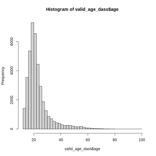
Looks good! Now it is always a good idea to inspect the values you removed from the data, in order to make sure that you did not remove something you intended to keep, and to learn something about the data you removed.
Let’s first check how many rows of data we actually removed:
R
n_rows_original <- nrow(dass_data)

n_rows_valid_age <- nrow(valid_age_dass)

n_rows_removed <- n_rows_original - n_rows_valid_age

n_rows_removed
OUTPUT
[1] 7This seems okay! Only 7 removed cases out of almost 40000 entries is negligible. Nonentheless, let’s investigate this further.
R
impossible_age_data <- filter(dass_data, age < 0 | age > 100)
Now we have a dataset that contains only the few cases with invalid ages. We can just look at the ages first:
R
impossible_age_data$age
OUTPUT
[1] 223 1996 117 1998 115 1993 1991Now, let’s try investigating the a little deeper. Do the people with invalid entries in age have valid entries in the other columns? Try to figure this out by visually inspecting the data. Where are they from? Do the responses to other questions seem odd?
This is possible, but somewhat hard to do for data with 170 columns. Looking through all of them might make you a bit tired after the third investigation of invalid data. What we really need is to look at only a few columns that interest us.
Selecting columns
This is where the function select() comes in. It enables
us to only retain some columns from a dataset for further analysis. You
just give it the data as the first argument and then list all of the
columns you want to keep.
R
inspection_data_impossible_age <- select(
    impossible_age_data,
    age, country, engnat, testelapse
  )

inspection_data_impossible_age
OUTPUT
   age country engnat testelapse
1  223      MY      2        456
2 1996      MY      2        259
3  117      US      1        114
4 1998      MY      2        196
5  115      AR      2        238
6 1993      MY      2        232
7 1991      MY      2        240
Here, we can see that our original data is reduced to the four
columns we specified above
age, country, engnat, testelapse. Do any of them look
strange? What happened in the age column?
To me, none of the other entries seem strange, the time it took them to complete the survey is plausible, they don’t show a clear trend of being from the same country. It seems that some people mistook the age question and entered their year of birth instead. Later on, we can try to fix this.
But before we do that, there are some more things about
select() that we can learn. It is one of the most useful
functions in my daily life, as it allows me to keep only those columns
that I am actually interested in. And it has many more features than
just listing the columns!
For example, note that the last few columns of the data are all the
demographic information. This is starting with education
and ending with major.
To select everything from education to
major:
R
# colnames() gives us the names of the columns only
colnames(select(valid_age_dass, education:major))
OUTPUT
 [1] "education"             "urban"                 "gender"
 [4] "engnat"                "age"                   "screensize"
 [7] "uniquenetworklocation" "hand"                  "religion"
[10] "orientation"           "race"                  "voted"
[13] "married"               "familysize"            "major"
We can also select all character columns using
where():
R
colnames(select(valid_age_dass, where(is.character)))
OUTPUT
[1] "country" "major" Or we can select all columns that start with the letter “Q”:
R
colnames(select(valid_age_dass, starts_with("Q")))
OUTPUT
  [1] "Q1A"  "Q1I"  "Q1E"  "Q2A"  "Q2I"  "Q2E"  "Q3A"  "Q3I"  "Q3E"  "Q4A"
 [11] "Q4I"  "Q4E"  "Q5A"  "Q5I"  "Q5E"  "Q6A"  "Q6I"  "Q6E"  "Q7A"  "Q7I"
 [21] "Q7E"  "Q8A"  "Q8I"  "Q8E"  "Q9A"  "Q9I"  "Q9E"  "Q10A" "Q10I" "Q10E"
 [31] "Q11A" "Q11I" "Q11E" "Q12A" "Q12I" "Q12E" "Q13A" "Q13I" "Q13E" "Q14A"
 [41] "Q14I" "Q14E" "Q15A" "Q15I" "Q15E" "Q16A" "Q16I" "Q16E" "Q17A" "Q17I"
 [51] "Q17E" "Q18A" "Q18I" "Q18E" "Q19A" "Q19I" "Q19E" "Q20A" "Q20I" "Q20E"
 [61] "Q21A" "Q21I" "Q21E" "Q22A" "Q22I" "Q22E" "Q23A" "Q23I" "Q23E" "Q24A"
 [71] "Q24I" "Q24E" "Q25A" "Q25I" "Q25E" "Q26A" "Q26I" "Q26E" "Q27A" "Q27I"
 [81] "Q27E" "Q28A" "Q28I" "Q28E" "Q29A" "Q29I" "Q29E" "Q30A" "Q30I" "Q30E"
 [91] "Q31A" "Q31I" "Q31E" "Q32A" "Q32I" "Q32E" "Q33A" "Q33I" "Q33E" "Q34A"
[101] "Q34I" "Q34E" "Q35A" "Q35I" "Q35E" "Q36A" "Q36I" "Q36E" "Q37A" "Q37I"
[111] "Q37E" "Q38A" "Q38I" "Q38E" "Q39A" "Q39I" "Q39E" "Q40A" "Q40I" "Q40E"
[121] "Q41A" "Q41I" "Q41E" "Q42A" "Q42I" "Q42E"
There are a number of helper functions you can use within
select():
-
starts_with("abc"): matches names that begin with “abc”. -
ends_with("xyz"): matches names that end with “xyz”. -
contains("ijk"): matches names that contain “ijk”. -
num_range("x", 1:3): matchesx1,x2andx3.
You can also remove columns using select by simply negating the
argument using !:
R
colnames(select(valid_age_dass, !starts_with("Q")))
OUTPUT
 [1] "country"               "source"                "introelapse"
 [4] "testelapse"            "surveyelapse"          "TIPI1"
 [7] "TIPI2"                 "TIPI3"                 "TIPI4"
[10] "TIPI5"                 "TIPI6"                 "TIPI7"
[13] "TIPI8"                 "TIPI9"                 "TIPI10"
[16] "VCL1"                  "VCL2"                  "VCL3"
[19] "VCL4"                  "VCL5"                  "VCL6"
[22] "VCL7"                  "VCL8"                  "VCL9"
[25] "VCL10"                 "VCL11"                 "VCL12"
[28] "VCL13"                 "VCL14"                 "VCL15"
[31] "VCL16"                 "education"             "urban"
[34] "gender"                "engnat"                "age"
[37] "screensize"            "uniquenetworklocation" "hand"
[40] "religion"              "orientation"           "race"
[43] "voted"                 "married"               "familysize"
[46] "major"
Now we will only get those columns that don’t start with “Q”.
Selecting a column twice
You can also use select to reorder the columns in your dataset. For example, notice that the following two bits of code return differently order data:
R
# head() gives us the first 10 values only
head(select(valid_age_dass, age, country, testelapse), 10)
OUTPUT
   age country testelapse
1   16      IN        167
2   16      US        193
3   17      PL        271
4   13      US        261
5   19      MY        164
6   20      US        349
7   17      MX      45459
8   29      GB        232
9   16      US        195
10  18      DE        120
R
head(select(valid_age_dass, testelapse, age, country), 10)
OUTPUT
   testelapse age country
1         167  16      IN
2         193  16      US
3         271  17      PL
4         261  13      US
5         164  19      MY
6         349  20      US
7       45459  17      MX
8         232  29      GB
9         195  16      US
10        120  18      DE
Using the function everything(), you can select all
columns.
What happens, when you select a column twice? Try running the following examples, what do you notice about the position of columns?
R
select(valid_age_dass, age, country, age)

select(valid_age_dass, age, country, everything())
Using the pipe %>%
Let’s retrace some of the steps that we took. We had the original
data dass_data and then filtered out those rows with
invalid entries in age. Then, we tried selecting only a couple of
columns in order to make the data more manageable. In code:
R
impossible_age_data <- filter(dass_data, age < 0 | age > 100)

inspection_data_impossible_age <- select(
  impossible_age_data,
  age, country, engnat, testelapse
  )
Notice how the first argument for both the filter() and
the select() function is always the data. This is also true
for the ggplot() function. And it’s no coincidence! In R,
there exists a special symbol, called the pipe %>%, that
has the following property: It takes the output of the previous function
and uses it as the first input in the following function.
This can make our example considerably easier to type:
R
dass_data %>%
  filter(age < 0 | age > 100) %>%
  select(age, country, engnat, testelapse)
OUTPUT
   age country engnat testelapse
1  223      MY      2        456
2 1996      MY      2        259
3  117      US      1        114
4 1998      MY      2        196
5  115      AR      2        238
6 1993      MY      2        232
7 1991      MY      2        240
Notice how the pipe is always written at the end of a line. This
makes it easier to understand and to read. As we go to the next line,
whatever is outputted is used as input in the following line. So the
original data dass_data is used as the first input in the
filter function, and the filtered data is used as the first input in the
select function.
To use the pipe, you can either type it out yourself or use the
Keyboard-Shortcut Ctrl + Shift + M.
Plotting using the pipe
We have seen that the pipe %>% allows us to chain
multiple functions together, making our code cleaner and easier to read.
This can be particularly useful when working with ggplot2,
where we often build plots step by step. Since ggplot()
takes the data as its first argument, we can use the pipe to make our
code more readable.
For example, let’s say we want to create a histogram of valid ages in our dataset. Instead of writing:
R
library(ggplot2)

ggplot(valid_age_dass, aes(x = age)) +
  geom_histogram(bins = 50)
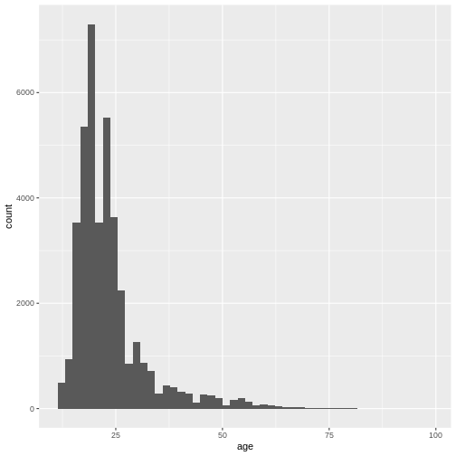
We can write:
R
valid_age_dass %>%
  ggplot(aes(x = age)) +
  geom_histogram(bins = 50)

This makes it clear that valid_age_dass is the dataset
being used, and it improves readability.
Using the pipe for the second argument
By default, the pipe places the output of the previous code as the
first argument in the following function. In most cases, this is exactly
what we want to have. If you want to be more explicit about where the
pipe should place the output, you can do this by placing a
. as the placeholder for piped-data.
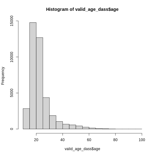
R
n_bins <- 30

n_bins %>%
  hist(valid_age_dass$age, .)
Numbered vs. Named Arguments
The pipe is made possible because most functions in the packages
included in tidyverse, like dplyr and
ggplot have the data as their first argument. This makes it
simple to pipe-through results from one function to the next, without
having to explicitly type function(data = something) every
time. In principle, almost all functions have a natural order in which
they expect arguments to occur. For example: ggplot()
expects data as the first argument and information about the mapping as
the second argument. This is why we always typed:
R
ggplot(
  data = valid_age_dass,
  mapping = aes(x = age)
)+
  geom_density()
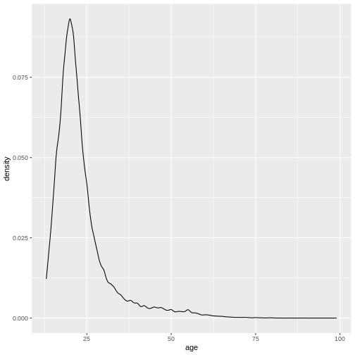
Notice that if we don’t specify the argument names, we still receive the same results. The function just uses the inputs you give it to match the arguments in the order in which they occur.
R
ggplot(
  valid_age_dass, # Now it just automatically thinks this is data =
  aes(x = age) # and this is mapping =
)+
  geom_density()

This is what makes this possible:
R
valid_age_dass %>%
  ggplot(aes(x = age)) +
  geom_density()

However, if we try to supply an argument in a place where it doesn’t belong, we get an error:
R
n_bins = 50
valid_age_dass %>%
  ggplot(aes(x = age)) +
  geom_histogram(n_bins)  # This will cause an error!
ERROR
Error in `geom_histogram()`:
! `mapping` must be created by `aes()`.
✖ You've supplied a number.
geom_histogram does not expect the number of bins to be
the first argument, but rather the mapping! Therefore, we need to
declare this properly:
R
valid_age_dass %>%
  ggplot(aes(x = age)) +
  geom_histogram(bins = n_bins)

To learn about the order of arguments of a function, use
?function and inspect the help file.
Common Problems
Using one pipe too little
A common mistake is forgetting to use a pipe between arguments of a chain. For example:
R
valid_age_dass %>%
  filter(age > 18)
  select(age, country)
Here, select() is not part of the pipeline because the
pipe is missing after filter(age > 18). This can lead to
unexpected errors or incorrect results. The correct way to write this
is:
R
valid_age_dass %>%
  filter(age > 18) %>%
  select(age, country)
Using one pipe too much
Another common problem is using one pipe too many without having a function following it.
ERROR
Error in parse(text = input): <text>:4:0: unexpected end of input
2:   filter(age > 18) %>%
3:   select(age, country) %>%
  ^
This can cause some really strange errors that never say anything about the pipe being superfluous. Make sure that all your pipe “lead somewhere”.
Using a pipe instead of + for
ggplot()
A source of confusion stems from the difference between the pipe
%>% and ggplot2’s +. They both
serve very similar purposes, namely adding together a chain of
functions. However, make sure you use %>% for everything
except ggplot-functions. Here, you will also receive an error
that is a little more informative:
R
valid_age_dass %>%
  ggplot(aes(x = age)) %>%
  geom_density()
ERROR
Error in `geom_density()` at magrittr/R/pipe.R:136:3:
! `mapping` must be created by `aes()`.
✖ You've supplied a <ggplot2::ggplot> object.
ℹ Did you use `%>%` or `|>` instead of `+`?
Using = Instead of == in
filter()
Another common error is using = instead of
== when filtering data. For example:
R
valid_age_dass %>%
  filter(country = "US") %>%  # Incorrect!
  head()
ERROR
Error in `filter()`:
! We detected a named input.
ℹ This usually means that you've used `=` instead of `==`.
ℹ Did you mean `country == "US"`?
This will result in an error because = is used for
assigning values, while == is used for comparisons. The
correct syntax is:
R
valid_age_dass %>%
  filter(country == "US") %>%
  select(country, engnat, education) %>%
  head()
OUTPUT
  country engnat education
1      US      1         2
2      US      1         1
3      US      2         2
4      US      2         2
5      US      1         1
6      US      1         2
Challenges
Challenge 1
Filter the complete dass_data. Create one dataset
containing only entries with people from the United States and one
dataset containing only entries from Great Britain. Compare the number
of entries in each dataset. What percentage of the total submissions
came from these two countries?
What is the average age of participants from the two countries?
Challenge 2
Create a filtered dataset based on the following conditions:
- The participant took less than 30 minutes to complete the DASS-part of the survey
- English is the native language of the participant
- There is an entry in the field
major
Challenge 3
What arguments does the cut() function take? Make a list
of the arguments and the order in which they have to be provided to the
function.
Challenge 4
In a single chain of functions, create a dataset is filtered with the same conditions as above and contains only the following variables:
- all demographic information, country information and the duration of the tests
- all the answers to the DASS (and only the answers, not the position or timing)
R
english_unversity_dass <- dass_data %>%
  filter(testelapse < 1800) %>%
  filter(engnat == 1) %>%
  filter(major != "") %>%
  select(starts_with("Q") & ends_with("A"), contains("elapse"), country, education:major)

write.csv(english_unversity_dass, "data/english_university_dass_data.csv")
Challenge 5
Save that dataset to a file
english_university_dass_data.csv in your
processed_data folder. You may need to use Google to find a
function that you can use to save data.
- Use the pipe operator
%>%to link multiple functions together - Use
filter()to filter rows based on certain conditions - Use
select()to keep only those rows that interest you