Vectors and variable types
Last updated on 2025-12-23 | Edit this page
Estimated time: 25 minutes
Overview
Questions
- How do you use scripts in R to document your work?
- How can you organize scripts effectively?
- What is a vector?
Objectives
- Show how to use scripts to generate reproducible analyses
- Explain what a vector is
- Explain variable types
- Show examples of
sum()andmean()
Scripts in R
For now, we have been only using the R console to execute commands. This works great if there are some quick calculations you have to run, but is unsuited for more complex analyses. If you want to reproduce the exact steps you took in data cleaning and analyses, you need to write them down - like a recipe.
This is where R scripts come in. They are basically like a text file (similar to Word) where you can write down all the steps you took. This makes it possible to retrace them and produce the exact same result over and over again.
In order to use R scripts effectively, you need to do two things.
Firstly, you need to write them in a way that is understandable in the
future. We will learn more about how to write clean code in future
lessons. Secondly (and maybe more importantly) you need to actually
save these scripts on your computer, and ideally save
them in a place where you can find them again. The place where you save
your script and especially the place you save your data should ideally
be a folder in a sensible place. For example, this script is saved in a
sub-folder episodes/ of the workshop folder
r_for_empra/. This makes it easy for humans to find the
script. Aim for similar clarity in your folder structure!
For this lesson, create a folder called r_for_empra
somewhere on your computer where it makes sense for you. Then, create a
new R script by clicking File > New File > R Script
or hitting Ctrl + Shift + N. Save this script as
episode_scripts_and_vectors.R in the folder
r_for_empra created above. Follow along with the episode
and note down the commands in your script.
Using a script
Let’s start learning about some basic elements of R programming. We
have already tried assigning values to variables using the
<- operator. For example, we might assign the constant
km_to_m the value 1000.
R
km_to_m <- 1000
Now, if we had data on distances in km, we could also use this value to compute the distance in meters.
R
distance_a_to_b_km <- 7.56

distance_a_to_b_m <- distance_a_to_b_km * km_to_m
If we have multiple distances and want to transform them from km to m
at the same time, we can make use of a vector. A vector is just a
collection of elements. We can create a vector using the function
c() (for combine).
Tip: Running segments of your code
RStudio offers you great flexibility in running code from within the
editor window. There are buttons, menu choices, and keyboard shortcuts.
To run the current line, you can 1. click on the Run button
just above the editor panel, or 2. select “Run Lines” from the “Code”
menu, or 3. hit Ctrl + Enter in Windows or Linux or
Command-Enter on OS X. (This shortcut can also be seen by hovering the
mouse over the button). To run a block of code, select it and then
Run via the button or the keyboard-shortcut
Ctrl + Enter.
Variable Types
Vectors can only contain values of the same type. There are two basic types of variables that you will have to interact with - numeric and character variables. Numeric variables are any numbers, character variables are bits of text.
R
# These are numeric variables:
vector_of_numeric_variables <- c(4, 7.642, 9e5, 1/97) # recall, 9e5 = 9*10^5

# Show the output
vector_of_numeric_variables
OUTPUT
[1] 4.000000e+00 7.642000e+00 9.000000e+05 1.030928e-02R
# These are character variables:
vector_of_character_variables <- c("This is a character variable", "A second variable", "And another one")

# Show the output
vector_of_character_variables
OUTPUT
[1] "This is a character variable" "A second variable"
[3] "And another one"
We can not only combine single elements into a vector, but also combine multiple vectors into one long vector.
R
numeric_vector_1 <- c(1, 2, 3, 4, 5)
numeric_vector_2 <- c(6:10) # 6:10 generates the values 6, 7, 8, 9, 10

combined_vector <- c(numeric_vector_1, numeric_vector_2)
combined_vector
OUTPUT
[1] 1 2 3 4 5 6 7 8 9 10Recall that all elements have to be of the same type. If you try to combine numeric vectors with character vectors, R will automatically convert everything to a character vector (as this has less restrictions, anything can be a character).
R
character_vector_1 <- c("6", "7", "8")
# Note that the numbers are now in quotation marks!
# They will be treated as characters, not numerics!

combining_numeric_and_character <- c(numeric_vector_1, character_vector_1)
combining_numeric_and_character
OUTPUT
[1] "1" "2" "3" "4" "5" "6" "7" "8"We can fix this issue by converting the vectors to the same type. Note how the characters are also just numbers, but in quotation marks. Sometimes, this happens in real data, too. Some programs store every variable as a character (sometimes also called string). We then have to convert the numbers back to the number format:
R
converted_character_vector_1 <- as.numeric(character_vector_1)

combining_numeric_and_converted_character <- c(numeric_vector_1, converted_character_vector_1)

combining_numeric_and_converted_character
OUTPUT
[1] 1 2 3 4 5 6 7 8But be careful, this conversion does not always work! If R does not
know how to convert a specific character to a number, it will simply
replace this with NA.
R
character_vector_2 <- c("10", "11", "text")
# The value "text", can not be interpreted as a number

as.numeric(character_vector_2)
WARNING
Warning: NAs introduced by coercionOUTPUT
[1] 10 11 NAInspecting the type of a variable
You can use the function str() to learn about the
structure of a variable. The first entry of the output tells us about
the type of the variable.
R
str(vector_of_numeric_variables)
OUTPUT
num [1:4] 4.00 7.64 9.00e+05 1.03e-02This tells us that there is a numeric vector, hence num, with 4 elements.
R
str(vector_of_character_variables)
OUTPUT
chr [1:3] "This is a character variable" "A second variable" ...This tells us that there is a character vector, hence chr, with 3 elements.
R
str(1:5)
OUTPUT
int [1:5] 1 2 3 4 5Note that this prints int and not the usual num. This is because the vector only contains integers, so whole numbers. These are stored in a special type that takes up less memory, because the numbers need to be stored with less precision. You can treat it as very similar to a numeric vector, and do all the same wonderful things with it!
Simple functions for vectors
Let’s use something more exciting than a sequence from 1 to 10 as an
example vector. Here, we use the mtcars data that you
already got to know in an earlier lesson. mtcars carries
information about cars, like their name, fuel usage, weight, etc. This
information is stored in a data frame. A data frame is a
rectangular collection of variables (in the columns) and observations
(in the rows). In order to extract vectors from a data frame we can use
the $ operator. data$column extracts a
vector.
R
mtcars_weight_tons <- mtcars$wt

# note that it is a good idea to include the unit in the variable name
mtcars_weight_tons
OUTPUT
 [1] 2.620 2.875 2.320 3.215 3.440 3.460 3.570 3.190 3.150 3.440 3.440 4.070
[13] 3.730 3.780 5.250 5.424 5.345 2.200 1.615 1.835 2.465 3.520 3.435 3.840
[25] 3.845 1.935 2.140 1.513 3.170 2.770 3.570 2.780
Let’s start learning some basic information about this vector:
R
str(mtcars_weight_tons)
OUTPUT
num [1:32] 2.62 2.88 2.32 3.21 3.44 ...The vector is of type numeric and contains 32 entries. We can double
check this by looking into our environment tab, where
num [1:32] indicates just that. Similarly, we can get the
length of a vector by using length()
R
length(mtcars_weight_tons)
OUTPUT
[1] 32We can compute some basic descriptive information of the weight of
cars in the mtcars data using base-R functions:
R
# Mean weight:
mean(mtcars_weight_tons)
OUTPUT
[1] 3.21725R
# Median weight:
median(mtcars_weight_tons)
OUTPUT
[1] 3.325R
# Standard deviation:
sd(mtcars_weight_tons)
OUTPUT
[1] 0.9784574To get the minimum and maximum value, we can use min()
and max().
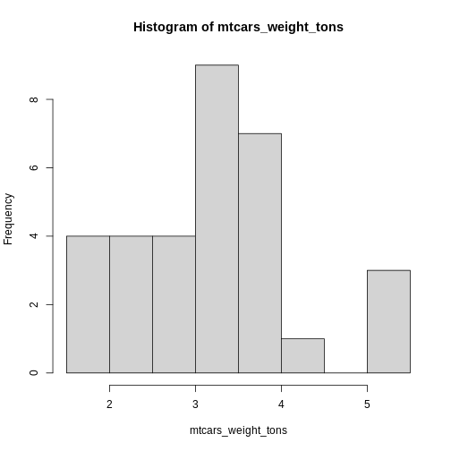
We can also get a quick overview of the weight distribution using
hist(), which generates a simple histogram.
R
hist(mtcars_weight_tons)
Histograms
Histograms are more powerful tools than it seems on first glance. They allow you to simply gather knowledge about the distribution of your data. This is especially important for us psychologists. Do we have ceiling effects in the task? Were some response options even used? How is response time distributed?
If your histogram is not detailed enough, try adjusting the
breaks parameter. This tells hist() how many
bars to print in the plot.
R
hist(mtcars_weight_tons, breaks = 30)
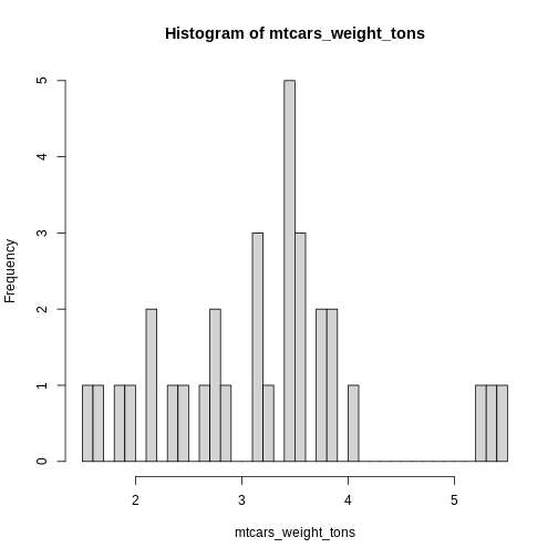
The golden rule for the number of breaks is simple: try it until it looks good! You are free to explore here.
Another useful function is unique(). This function
removes duplicates and only returns unique values. I use it a lot in
experimental data. Since every participant contributes multiple trials,
but I am sometimes interested in values a participant only contributes
once, I can use unique() to only retain each value
once.
In mtcars data, we might want to see how many cylinders
are possible in the data. unique(mtcars$cyl) is much easier
to read at a glance.
R
mtcars$cyl
OUTPUT
[1] 6 6 4 6 8 6 8 4 4 6 6 8 8 8 8 8 8 4 4 4 4 8 8 8 8 4 4 4 8 6 8 4R
unique(mtcars$cyl)
OUTPUT
[1] 6 4 8Tip: Unique + Length = Quick Count
Combining unique() and length() leads to a
really useful property. This returns the number of unique entries in a
vector. I use it almost daily! For example to figure out how many
participants are in a given data frame.
unique(data$participant_id) returns all the different
participant ids and length(unique(data$participant_id))
then gives me the number of different ids, so the number of participants
in my data.
Indexing and slicing vectors
There is one more important thing to learn about vectors before we move on to more complicated data structures. Most often, you are going to use the whole vector for computation. But sometimes you may only want the first 150 entries, or only entries belonging to a certain group. Here, you must be able to access specific elements of the vector.
In the simplest case, you can access the \(n\)th element in a vector by using
vector[n]. To access the first entry, use
vector[1], and so on.
R
test_indexing_vector <- seq(1, 32, 1)
# Seq generates a sequence from the first argument (1) to the second argument (32)
# The size of the steps is given by the third argument

test_indexing_vector
OUTPUT
 [1]  1  2  3  4  5  6  7  8  9 10 11 12 13 14 15 16 17 18 19 20 21 22 23 24 25
[26] 26 27 28 29 30 31 32
R
test_indexing_vector[1]
OUTPUT
[1] 1R
test_indexing_vector[c(1, 2)]
OUTPUT
[1] 1 2You can also remove an element (or multiple) from a vector by using a
negative sign -.
R
test_indexing_vector[-c(11:32)] # this removes all indexes from 11 to 32
OUTPUT
[1] 1 2 3 4 5 6 7 8 9 10The same rules apply for all types of vectors (numeric and character).
Tip: Think about the future
Excluding by index is a simple way to clean vectors. However, think
about what happens if you accidentally run the command
vector <- vector[-1] twice, instead of once?
The first element is going to be excluded twice. This means that the vector will lose two elements. In principle, it is a good idea to write code that you can run multiple times without causing unwanted issues. To achieve this, either use a different way to exclude the first element that we will talk about later, or simply assign the cleaned vector a new name:
R
cleaned_vector <- vector[-1]
Now, no matter how often you run this piece of code,
cleaned_vector will always be vector without
the first entry.
Filtering vectors
In most cases, you don’t know what the element of the vector is you want to exclude. You might know that some values are impossible or not of interest, but don’t know where they are. For example, the accuracy vector of a response time task might look like this:
R
accuracy_coded <- c(0, 1, 1, 1, 1, -2, 99, 1, 11, 0)
accuracy_coded
OUTPUT
[1] 0 1 1 1 1 -2 99 1 11 0-2 and 99 are often used to indicate
invalid button-presses or missing responses. 11 in this
case is a wrong entry that should be corrected to 1.
If we were to compute the average accuracy now using
mean() we would receive a wrong response.
R
mean(accuracy_coded)
OUTPUT
[1] 11.3Therefore, we need to exclude all invalid values before continuing our analysis. Before I show you how I would go about doing this, think about it yourself. You do not need to know the code, yet. Just think about some rules and steps that need to be taken to clean up the accuracy vector. What comparisons could you use?
Important: The silent ones are the worst
The above example illustrates something very important. R will not
throw an error every time you do something that doesn’t make sense. You
should be really careful of “silent” errors. The mean()
function above works exactly as intended, but returns a completely
nonsensical value. You should always conduct sanity checks. Can
mean accuracy be higher than 1? How many entries am I expecting in my
data?
Now, back to the solution to the wacky accuracy data. Note that R gives us the opportunity to do things in a million different ways. If you came up with something different from what was presented here, great! Make sure it works and if so, use it!
First, we need to recode the wrong entry. That 11 was
supposed to be a 1, but someone entered the wrong data in
the excel. To do this, we can find the index, or the element number,
where accuracy is 11. Then, we can replace that entry with 1.
R
index_where_accuracy_11 <- which(accuracy_coded == 11)

accuracy_coded[index_where_accuracy_11] <- 1
# or in one line:
# accuracy_coded[which(accuracy_coded == 11)] <- 1

accuracy_coded
OUTPUT
[1] 0 1 1 1 1 -2 99 1 1 0Now, we can simply exclude all values that are not equal to 1 or 0.
We do this using the - operators:
R
accuracy_coded[-which(accuracy_coded != 0 & accuracy_coded != 1)]
OUTPUT
[1] 0 1 1 1 1 1 1 0However, note that this reduces the number of entries we have in our
vector. This may not always be advisable. Therefore, it is often better
to replace invalid values with NA. The value
NA (not available) indicates that something is not a
number, but just missing.
R
# Note that now we are not using the - operator
# We want to replace values that are not 0 or 1
accuracy_coded[which(accuracy_coded != 0 & accuracy_coded != 1)] <- NA
Now, we can finally compute the average accuracy in our fictional experiment.
R
mean(accuracy_coded)
OUTPUT
[1] NAChallenges
Challenge 1:
We did not get a number in the above code. Figure out why and how to fix this. You are encourage to seek help on the internet.
Challenge 2:
Below is a vector of response times. Compute the mean response time, the standard deviation, and get the number of entries in this vector.
R
response_times_ms <- c(
  230.7298, 620.6292, 188.8168, 926.2940, 887.4730,
  868.6299, 834.5548, 875.2154, 239.7057, 667.3095,
  -142.891, 10000, 876.9879
  )
Challenge 3:
There might be some wrong values in the response times vector from
above. Use hist() to inspect the distribution of response
times. Figure out which values are implausible and exclude them.
Recompute the mean response time, standard deviation, and the number of
entries.
Challenge 4:
Get the average weight (column wt) of cars in the
mtcars data . Can you spot any outliers in the
histogram?
Exclude the “outlier” and rerun the analyses.
Challenge 5:
Get the mean values of responses to this fictional questionnaire:
R
item_15_responses <- c("1", "3", "2", "1", "2", "none", "4", "1", "3", "2", "1", "1", "none")
Challenge 6 (difficult):
Compute the average of responses that are valid as indicated by the
vector is_response_valid:
R
response_values <- c(91, 82, 69, 74, 62, 19, 84, 61, 92, 53)
is_response_valid <- c("yes", "yes", "yes", "yes", "yes",
                       "no", "yes", "yes", "yes", "no")
R
valid_responses <- response_values[which(is_response_valid == "yes")]
mean(valid_responses)
OUTPUT
[1] 76.875- Scripts facilitate reproducible research
- create vectors using
c() - Numeric variables are used for computations, character variables often contain additional information
- You can index vectors by using
vector[index]to return or exclude specific indices - Use
which()to filter vectors based on specific conditions